All in One View
Content from Introduction to RNA-seq
Last updated on 2026-06-16 | Edit this page
Estimated time: 100 minutes
Overview
Questions
- What are the different choices to consider when planning an RNA-seq experiment?
- How does one process the raw fastq files to generate a table with read counts per gene and sample?
- Where does one find information about annotated genes for a given organism?
- What are the typical steps in an RNA-seq analysis?
Objectives
- Explain what RNA-seq is.
- Describe some of the most common design choices that have to be made before running an RNA-seq experiment.
- Provide an overview of the procedure to go from the raw data to the read count matrix that will be used for downstream analysis.
- Show some common types of results and visualizations generated in RNA-seq analyses.
What are we measuring in an RNA-seq experiment?
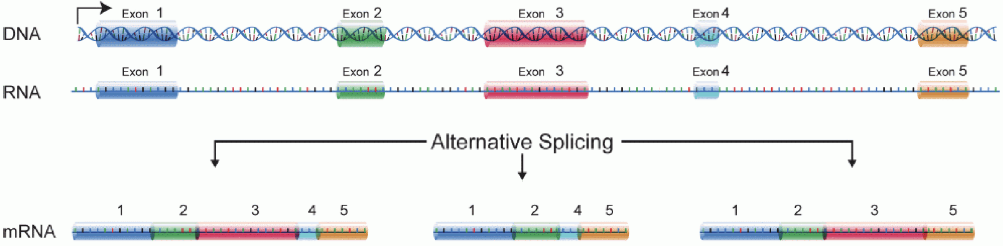
In order to produce an RNA molecule, a stretch of DNA is first transcribed into mRNA. Subsequently, intronic regions are spliced out, and exonic regions are combined into different isoforms of a gene.
(figure adapted from Martin & Wang (2011)).
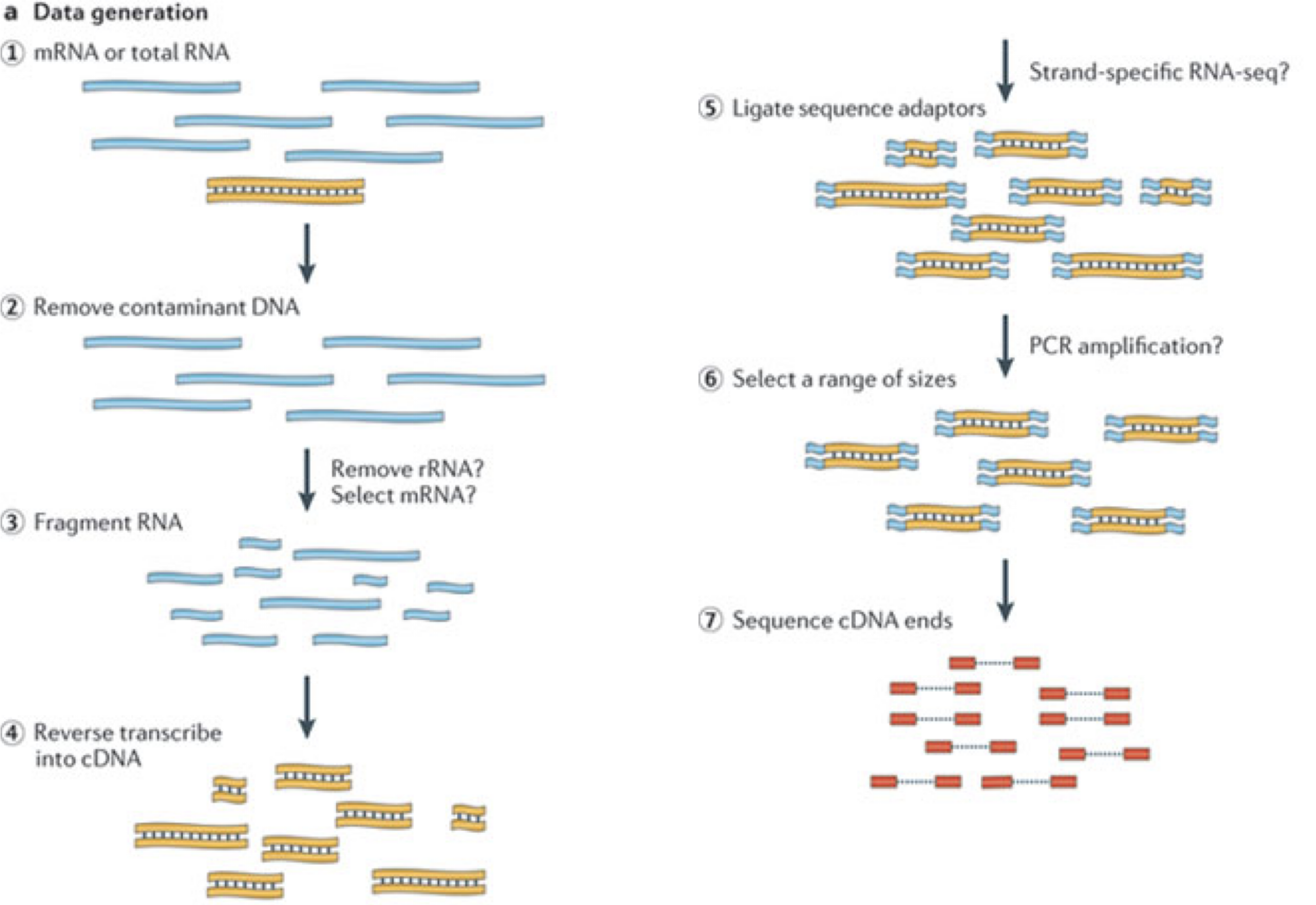
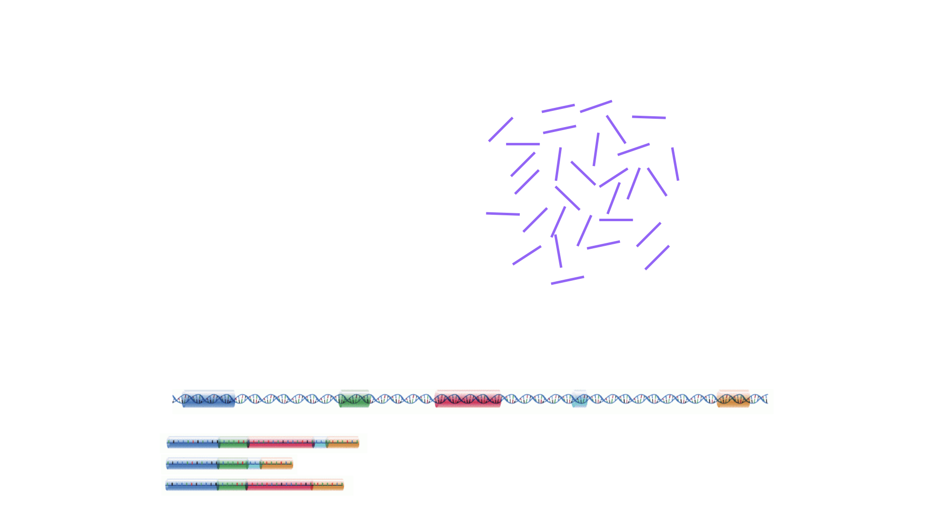
In a typical RNA-seq experiment, RNA molecules are first collected from a sample of interest. After a potential enrichment for molecules with polyA tails (predominantly mRNA), or depletion of otherwise highly abundant ribosomal RNA, the remaining molecules are fragmented into smaller pieces (there are also long-read protocols where entire molecules are considered, but those are not the focus of this lesson). It is important to keep in mind that because of the splicing excluding intronic sequences, an RNA molecule (and hence a generated fragment) may not correspond to an uninterrupted region of the genome. The RNA fragments are then reverse transcribed into cDNA, whereafter sequencing adapters are added to each end. These adapters allow the fragments to attach to the flow cell. Once attached, each fragment will be heavily amplified to generate a cluster of identical sequences on the flow cell. The sequencer then determines the sequence of the first 50-200 nucleotides of the cDNA fragments in each such cluster, starting from one end, which corresponds to a read. Many data sets are generated with so called paired-end protocols, in which the fragments are read from both ends. Millions of such reads (or pairs of reads) will be generated in an experiment, and these will be represented in a (pair of) FASTQ files. Each read is represented by four consecutive lines in such a file: first a line with a unique read identifier, next the inferred sequence of the read, then another identifier line, and finally a line containing the base quality for each inferred nucleotide, representing the probability that the nucleotide in the corresponding position has been correctly identified.
Challenge: Discuss the following points with your neighbor
- What are potential advantages and disadvantages of paired-end protocols compared to only sequencing one end of a fragment?
- What quality assessment can you think of that would be useful to perform on the FASTQ files with read sequences?
Experimental design considerations
Before starting to collect data, it is essential to take some time to think about the design of the experiment. Experimental design concerns the organization of experiments with the purpose of making sure that the right type of data, and enough of it, is available to answer the questions of interest as efficiently as possible. Aspects such as which conditions or sample groups to consider, how many replicates to collect, and how to plan the data collection in practice are important questions to consider. Many high-throughput biological experiments (including RNA-seq) are sensitive to ambient conditions, and it is often difficult to directly compare measurements that have been done on different days, by different analysts, in different centers, or using different batches of reagents. For this reason, it is very important to design experiments properly, to make it possible to disentangle different types of (primary and secondary) effects.
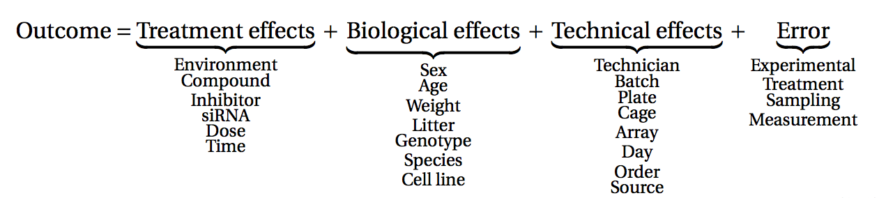
(figure from Lazic (2017)).
Challenge: Discuss with your neighbor
- Why is it essential to have replicates?
Importantly, not all replicates are equally useful, from a statistical point of view. One common way to classify the different types of replicates is as ‘biological’ and ‘technical’, where the latter are typically used to test the reproducibility of the measurement device, while biological replicates inform about the variability between different samples from a population of interest. Another scheme classifies replicates (or units) into ‘biological’, ‘experimental’ and ‘observational’. Here, biological units are entities we want to make inferences about (e.g., animals, persons). Replication of biological units is required to make a general statement of the effect of a treatment - we can not draw a conclusion about the effect of drug on a population of mice by studying a single mouse only. Experimental units are the smallest entities that can be independently assigned to a treatment (e.g., animal, litter, cage, well). Only replication of experimental units constitute true replication. Observational units, finally, are entities at which measurements are made.
To explore the impact of experimental design on the ability to answer questions of interest, we are going to use an interactive application, provided in the ConfoundingExplorer package.
Challenge
Launch the ConfoundingExplorer application and familiarize yourself with the interface.
Challenge
- For a balanced design (equal distribution of replicates between the two groups in each batch), what is the effect of increasing the strength of the batch effect? Does it matter whether one adjusts for the batch effect or not?
- For an increasingly unbalanced design (most or all replicates of one group coming from one batch), what is the effect of increasing the strength of the batch effect? Does it matter whether one adjusts for the batch effect or not?
RNA-seq quantification: from reads to count matrix
The read sequences contained in the FASTQ files from the sequencer are typically not directly useful as they are, since we do not have the information about which gene or transcript they originate from. Thus, the first processing step is to attempt to identify the location of origin for each read, and use this to obtain an estimate of the number of reads originating from a gene (or another features, such as an individual transcript). This can then be used as a proxy for the abundance, or expression level, of the gene. There is a plethora of RNA quantification pipelines, and the most common approaches can be categorized into three main types:
Align reads to the genome, and count the number of reads that map within the exons of each gene. This is the one of simplest methods. For species for which the transcriptome is poorly annotated, this would be the preferred approach. Example:
STARalignment to GRCm39 +RsubreadfeatureCountsAlign reads to the transcriptome, quantify transcript expression, and summarize transcript expression into gene expression. This approach can produce accurate quantification results (independent benchmarking), particularly for high-quality samples without DNA contamination. Example: RSEM quantification using
rsem-calculate-expression --staron the GENCODE GRCh38 transcriptome +tximportPseudoalign reads against the transcriptome, using the corresponding genome as a decoy, quantifying transcript expression in the process, and summarize the transcript-level expression into gene-level expression. The advantages of this approach include: computational efficiency, mitigation of the effect of DNA contamination, and GC bias correction. Example:
salmon quant --gcBias+tximport
At typical sequencing read depth, gene expression quantification is often more accurate than transcript expression quantification. However, differential gene expression analyses can be improved by having access also to transcript-level quantifications.
Other tools used in RNA-seq quantification include: TopHat2, Bowtie2, Kallisto, HTSeq, among many others.
The choice of an appropriate RNA-seq quantification depends on the quality of the transcriptome annotation, the quality of the RNA-seq library preparation, the presence of contaminating sequences, among many factors. Often, it can be informative to compare the quantification results of multiple approaches.
The quantification method is species- and experiment-dependent, and often requires large amounts of computing resources, so we will give you a overview of how to perform quantification, and scripts to run the quantification. We will use pre-computed quantifications for the exercises in this workshop.
Challenge: Discuss the following points with your neighbor
- Which of the mentioned RNA-Seq quantification tools have you heard about? Do you know other pros and cons of the methods?
- Have you done your own RNA-Seq experiment? If so, what quantification tool did you use and why did you choose it?
- Do you have access to specific tools / local bioinformatics expert / computational resources for quantification? If you don’t, how might you gain access?
Finding the reference sequences
In order to quantify abundances of known genes or transcripts from RNA-seq data, we need a reference database informing us of the sequence of these features, to which we can then compare our reads. This information can be obtained from different online repositories. It is highly recommended to choose one of these for a particular project, and not mix information from different sources. Depending on the quantification tool you have chosen, you will need different types of reference information. If you are aligning your reads to the genome and investigating the overlap with known annotated features, you will need the full genome sequence (provided in a fasta file) and a file that tells you the genomic location of each annotated feature (typically provided in a gtf file). If you are mapping your reads to the transcriptome, you will instead need a file with the sequence of each transcript (again, a fasta file).
- If you are working with mouse or human samples, the GENCODE project provides well-curated reference files.
- Ensembl provides reference files for a large set of organisms, including plants and fungi.
- UCSC also provides reference files for many organisms.
Challenge
Download the latest mouse transcriptome fasta file from GENCODE. What
do the entries look like? Tip: to read the file into R, consider the
readDNAStringSet() function from the
Biostrings package.
Where are we heading towards in this workshop?
In this workshop, we will discuss and practice: downloading publicly available RNA-seq data, performing quality assessment of the raw data, quantifying gene expression, and performing differential expression analysis to identify genes that are expressed at different levels between two or more conditions. We will also cover some aspects of data visualization and interpretation of the results.
The outcome of a differential expression analysis is often represented using graphical representations, such as MA plots and heatmaps (see below for examples).
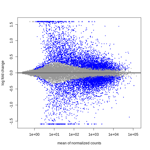
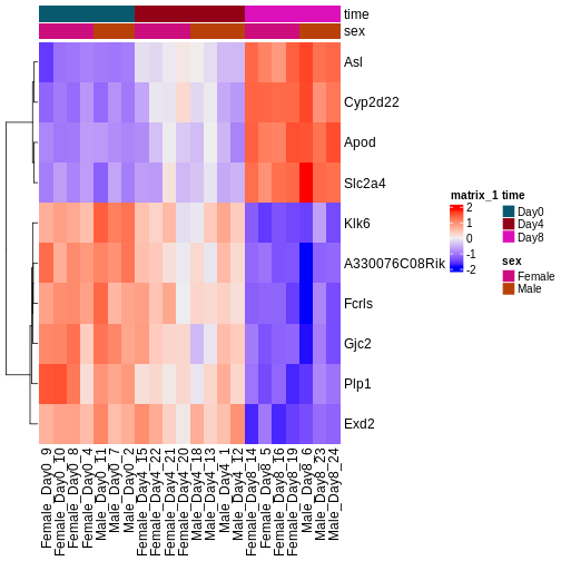
In the following episodes we will learn, among other things, how to generate and interpret these plots. It is also common to perform follow-up analyses to investigate whether there is a functional relationship among the top-ranked genes, so called gene set (enrichment) analysis, which will also be covered in a later episode.
- RNA-seq is a technique of measuring the amount of RNA expressed within a cell/tissue and state at a given time.
- Many choices have to be made when planning an RNA-seq experiment, such as whether to perform poly-A selection or ribosomal depletion, whether to apply a stranded or an unstranded protocol, and whether to sequence the reads in a single-end or paired-end fashion. Each of the choices have consequences for the processing and interpretation of the data.
- Many approaches exist for quantification of RNA-seq data. Some methods align reads to the genome and count the number of reads overlapping gene loci. Other methods map reads to the transcriptome and use a probabilistic approach to estimate the abundance of each gene or transcript.
- Information about annotated genes can be accessed via several sources, including Ensembl, UCSC and GENCODE.
Content from Downloading and organizing files
Last updated on 2026-06-16 | Edit this page
Estimated time: 35 minutes
Overview
Questions
- What files are required to process raw RNA seq reads?
- Where do we obtain raw reads, reference genomes, annotations, and transcript sequences?
- How should project directories be organized to support a smooth workflow?
- What practical considerations matter when downloading and preparing RNA seq data?
Objectives
- Identify the essential inputs for RNA seq analysis: FASTQ files, reference genome, annotation, and transcript sequences.
- Learn where and how to download RNA seq datasets and reference materials.
- Create a clean project directory structure suitable for quality control, alignment, and quantification.
- Understand practical issues such as compressed FASTQ files and adapter trimming.
Introduction
Before we can perform quality control, mapping, or quantification, we must first gather the files required for RNA seq analysis and organize them in a reproducible way. This episode introduces the essential inputs of an RNA seq workflow and demonstrates how to obtain and structure them on a computing system.
We begin by discussing raw FASTQ reads, reference genomes, annotation files, and transcript sequences. We then download the dataset used throughout the workshop and set up the directory structure that supports downstream steps.
Most FASTQ files arrive compressed as .fastq.gz files.
Modern RNA seq tools accept compressed files directly, so uncompressing
them is usually unnecessary.
Should I uncompress FASTQ files?
In almost all RNA-seq workflows, you should keep FASTQ files
compressed. Tools such as FastQC, HISAT2, STAR, Salmon, and fastp can
read .gz files directly. Keeping files compressed saves
space and reduces input and output overhead.
Many library preparation protocols introduce adapter sequences at the ends of reads. For most alignment based analyses, explicit trimming is not required because aligners soft clip adapter sequences automatically.
Should I trim adapters for RNA seq analysis?
In most cases, no. Aligners such as HISAT2 and STAR soft clip adapter
sequences. Overly aggressive trimming can reduce mapping rates or
distort read length distributions. Trimming is needed only for specific
applications such as transcript assembly where uniform read lengths are
important.
More information: https://www.ncbi.nlm.nih.gov/pmc/articles/PMC4766705/
The workshop dataset: p53-mediated response to ionizing radiation
For this workshop, we use a subset of a publicly available dataset (GEO accession GSE71176) that investigates the transcriptional response to ionizing radiation (IR) in mouse B cells. The original study by Tonelli et al. (2015) examined how the tumor suppressor p53 (encoded by Trp53) regulates gene expression following DNA damage.
Biological context
The TP53 gene (called Trp53 in mice) encodes the p53 protein, often called the “guardian of the genome.” When cells experience DNA damage, such as double-strand breaks caused by ionizing radiation, p53 activates transcriptional programs that lead to:
- Cell cycle arrest (allowing time for DNA repair)
- Apoptosis (programmed cell death if damage is irreparable)
- Senescence (permanent growth arrest)
- Metabolic reprogramming
Mutations in TP53 are among the most common alterations in human cancers, occurring in approximately 50% of all tumors. Understanding p53-regulated genes is therefore central to cancer biology.
Experimental design
The full dataset includes wild-type (WT) and p53-knockout (KO) mouse B cells, with and without IR treatment (7 Gy, 4 hours post-exposure). For simplicity, we will focus on 8 samples from wild-type B cells only:
| Condition | Description | Samples | Replicates |
|---|---|---|---|
| WT_mock (control) | Wild-type B cells, no radiation | 4 | SRR2121778-81 |
| WT_IR (treatment) | Wild-type B cells, 4h post 7Gy IR | 4 | SRR2121786-89 |
This balanced design (n=4 per group) allows us to identify genes that respond to ionizing radiation in cells with functional p53.
Expected biological results
Because p53 is a transcription factor activated by DNA damage, we expect to see upregulation of canonical p53 target genes in IR-treated samples:
Genes expected to be upregulated (IR vs mock):
- Cdkn1a (p21) - cell cycle arrest
- Bax, Bbc3 (Puma), Pmaip1 (Noxa) - pro-apoptotic
- Mdm2 - negative feedback regulator of p53
- Gadd45a - DNA damage response
- Fas, Tnfrsf10b (DR5) - death receptor signaling
Pathways expected to be enriched:
- p53 signaling pathway
- Apoptosis
- Cell cycle
- DNA damage response
The presence of these expected results serves as a positive control that our analysis pipeline is working correctly.
Why this dataset?
This dataset is ideal for teaching because:
- Simple two-group comparison: Control vs. treatment with balanced replicates
- Clear biological interpretation: DNA damage response is well-characterized
- Expected positive controls: Known p53 targets should appear as top hits
- Clinical relevance: p53 biology is fundamental to cancer research
- Model organism: Mouse with excellent genome annotation
Project organization
Before downloading files, we create a reproducible directory layout for raw data, scripts, mapping outputs, and count files.
Create the directories needed for this episode
Create a working directory for the workshop (e.g.,
rnaseq-workshop). Inside it, create four
subdirectories:
-
data: raw FASTQ files, reference genome, annotation
-
scripts: custom scripts, SLURM job files
-
results: alignment, counts and various other outputs
The resulting directory structure should look like this:
What files do I need for RNA-seq analysis?
You will need:
- Raw reads (FASTQ)
- Usually
.fastq.gzfiles containing nucleotide sequences and per-base quality scores.
- Usually
For alignment based workflows
- Reference genome (FASTA)
- Contains chromosome or contig sequences.
- Annotation file (GTF/GFF)
- Describes gene models: exons, transcripts, coordinates.
For transcript-level quantification workflows
- Transcript sequences (FASTA)
- Required for transcript-based quantification with tools such as Salmon, Kallisto, and RSEM.
Reference files must be consistent with each other (same genome version). To ensure a smooth analysis workflow, keep these files logically organized. Good directory structure minimizes mistakes, simplifies scripting, and supports reproducibility.
Downloading the data
We now download:
- the GRCm39 reference genome
- the corresponding GENCODE annotation
- transcript sequences (if using transcript based quantification)
- raw FASTQ files from SRA
Reference genome and annotation
We will use GENCODE GRCm39 (M38) as the reference.
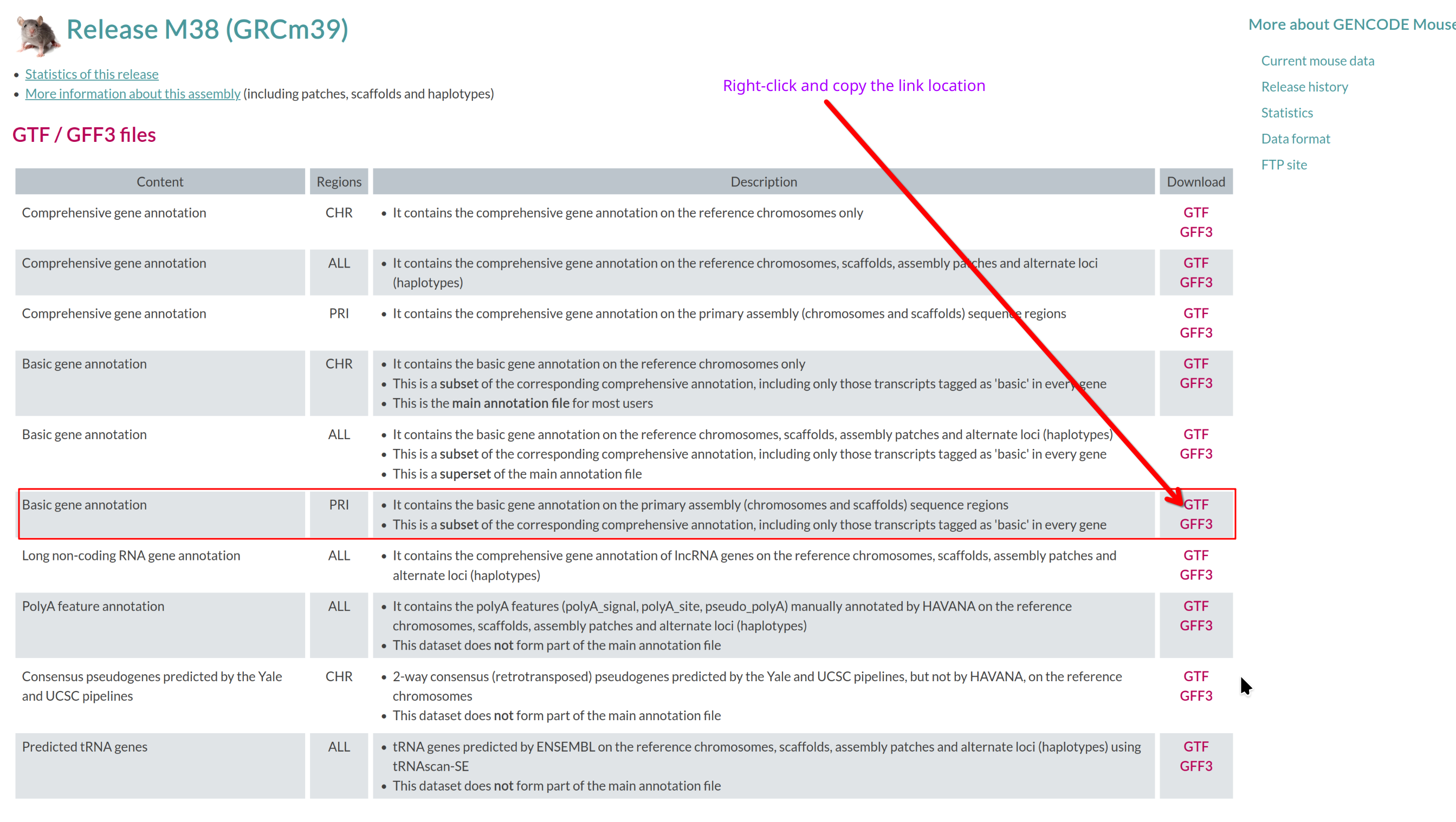
Annotation
Visit the GENCODE mouse page: https://www.gencodegenes.org/mouse/.
Which annotation file (GTF/GFF3 files section) should you download, and
why?
Use the basic gene annotation in GTF format (e.g.,
gencode.vM38.primary_assembly.basic.annotation.gtf.gz).
It contains essential gene and transcript models without pseudogenes or
other biotypes not typically used for RNA-seq quantification.
Reference genome
Select the corresponding Genome sequence (GRCm39)
FASTA (e.g.,
GRCm39.primary_assembly.genome.fa.gz).
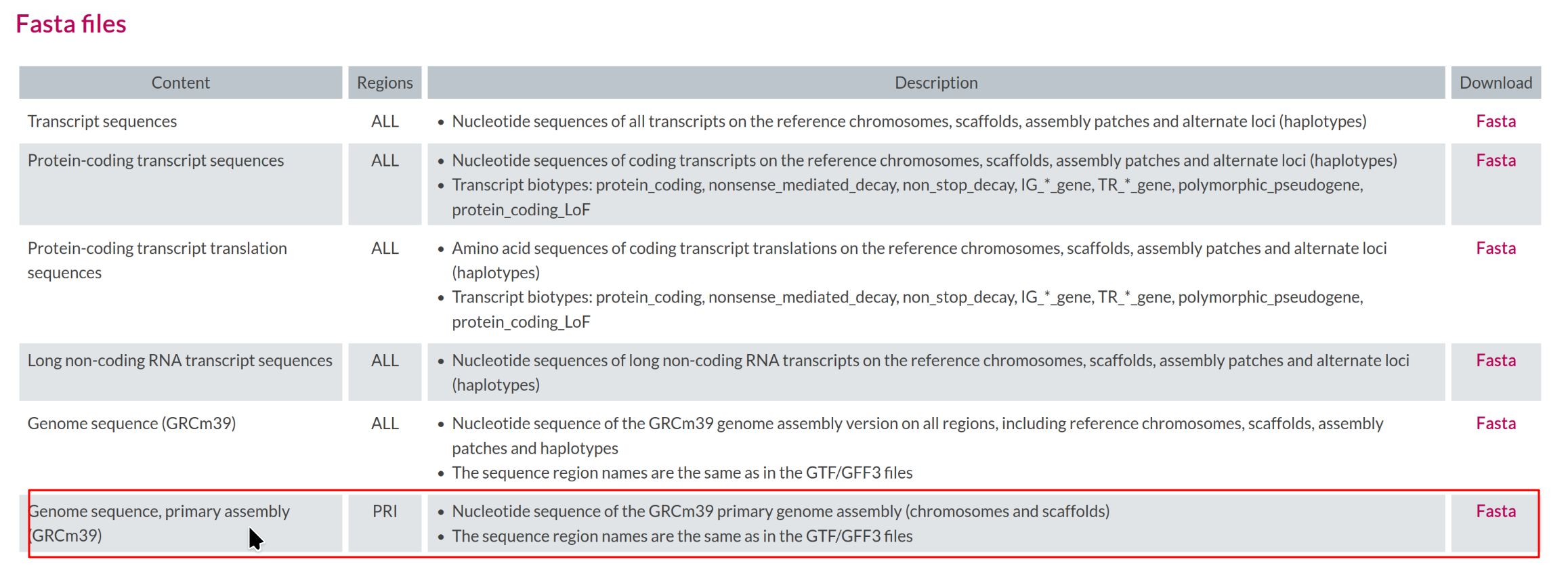
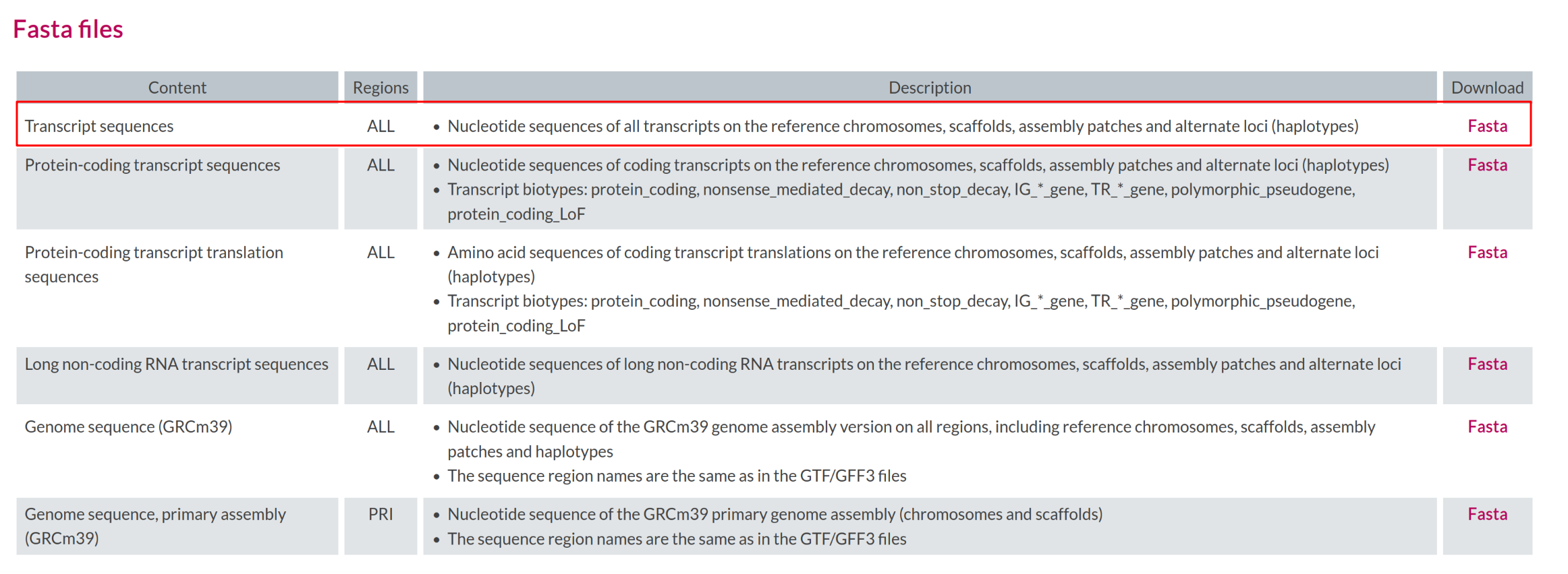
Transcript sequences
Transcript level quantification requires a transcript FASTA file
consistent with the annotation. GENCODE provides transcript sequences
for all transcripts in GRCm39
(gencode.vM38.transcripts.fa.gz).
Transcript sequence file
Where on the GENCODE page can you find the transcript FASTA file?
The transcript FASTA file is available in the same release directory
as the genome and annotation files (under FASTA files). It is named
gencode.vM38.transcripts.fa.gz.
Downloading all reference files
BASH
cd ${SCRATCH}/rnaseq-workshop

GTFlink="https://ftp.ebi.ac.uk/pub/databases/gencode/Gencode_mouse/release_M38/gencode.vM38.primary_assembly.basic.annotation.gtf.gz"
GENOMElink="https://ftp.ebi.ac.uk/pub/databases/gencode/Gencode_mouse/release_M38/GRCm39.primary_assembly.genome.fa.gz"
CDSLink="https://ftp.ebi.ac.uk/pub/databases/gencode/Gencode_mouse/release_M38/gencode.vM38.transcripts.fa.gz"

# Download to 'data'
wget -P data ${GENOMElink}
wget -P data ${GTFlink}
wget -P data ${CDSLink}

# Uncompress
cd data
gunzip GRCm39.primary_assembly.genome.fa.gz
gunzip gencode.vM38.primary_assembly.basic.annotation.gtf.gz
gunzip gencode.vM38.transcripts.fa.gz
The transcript file header has multiple pieces of information which often interfere with downstream analysis. We create a simplified version containing only the transcript IDs.
Raw reads
-
Study: Genome-wide analysis of p53 transcriptional
programs in B cells upon exposure to genotoxic stress in
vivo
- Organism: Mus musculus (C57BL/6)
- Cell type: Primary B cells from spleen
- Design: Wild-type mock vs Wild-type IR-treated (n=4 per group)
- Treatment: 7 Gy ionizing radiation, harvested 4 hours post-exposure
- Sequencing: Illumina HiSeq 2000, paired-end 51bp
- GEO: GSE71176
- Reference: Tonelli et al. Oncotarget 2015 Sep 22;6(28):24611-26. PMID: 26372730
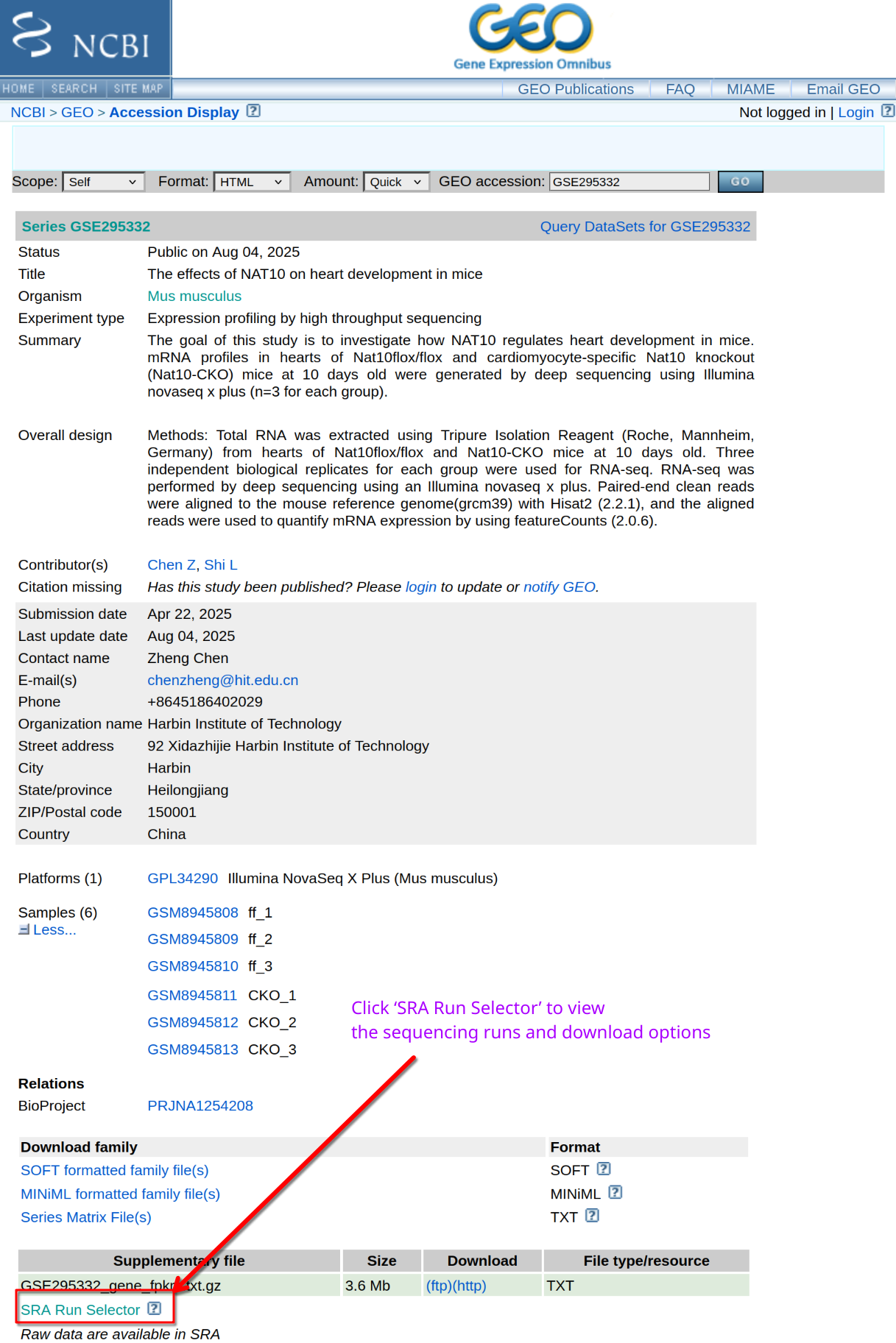
Where do you find FASTQ files?
GEO provides metadata and experimental details, but FASTQ files are stored in the SRA. How do you obtain the complete list of sequencing runs?
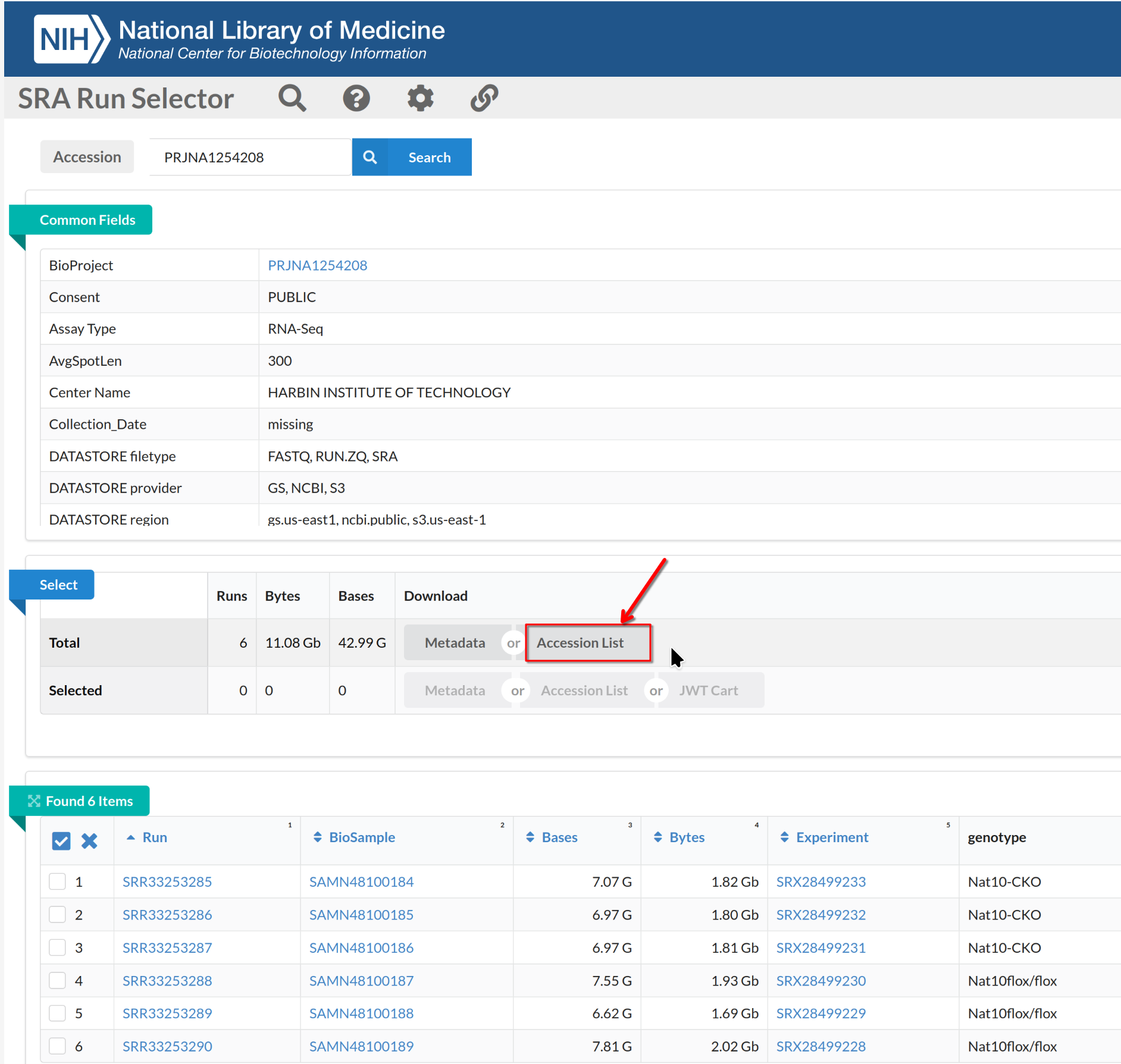
Navigate to the SRA page for the BioProject and use Run
Selector to list runs.
On the Run Selector page, select the accessions (SRR2121778-81,
SRR2121786-89), toggle the “selected” and click Accession
List to download the selected SRR accession IDs.
Download FASTQ files with SRA Toolkit
[DO NOT RUN THIS COMMAND DURING THE WORKSHOP - IT TAKES TOO LONG TO COMPLETE]. You already copied the pre-downloaded data to your scratch space.
BASH
sinteractive -A rcac-rnaseq -q standby -p cpu -N 1 -n 4 --time=1:00:00
cd ${SCRATCH}/rnaseq-workshop/data
module load biocontainers
module load sra-tools
while read SRR; do
   fasterq-dump --threads 4 --progress $SRR;
   gzip ${SRR}_1.fastq
   gzip ${SRR}_2.fastq
done<SRR_Acc_List.txt
# rename files to meaningful names
# WT B cells - mock
mv SRR2121778_1.fastq.gz WT_Bcell_mock_rep1_R1.fastq.gz
mv SRR2121778_2.fastq.gz WT_Bcell_mock_rep1_R2.fastq.gz
mv SRR2121779_1.fastq.gz WT_Bcell_mock_rep2_R1.fastq.gz
mv SRR2121779_2.fastq.gz WT_Bcell_mock_rep2_R2.fastq.gz
mv SRR2121780_1.fastq.gz WT_Bcell_mock_rep3_R1.fastq.gz
mv SRR2121780_2.fastq.gz WT_Bcell_mock_rep3_R2.fastq.gz
mv SRR2121781_1.fastq.gz WT_Bcell_mock_rep4_R1.fastq.gz
mv SRR2121781_2.fastq.gz WT_Bcell_mock_rep4_R2.fastq.gz
# WT B cells - IR
mv SRR2121786_1.fastq.gz WT_Bcell_IR_rep1_R1.fastq.gz
mv SRR2121786_2.fastq.gz WT_Bcell_IR_rep1_R2.fastq.gz
mv SRR2121787_1.fastq.gz WT_Bcell_IR_rep2_R1.fastq.gz
mv SRR2121787_2.fastq.gz WT_Bcell_IR_rep2_R2.fastq.gz
mv SRR2121788_1.fastq.gz WT_Bcell_IR_rep3_R1.fastq.gz
mv SRR2121788_2.fastq.gz WT_Bcell_IR_rep3_R2.fastq.gz
mv SRR2121789_1.fastq.gz WT_Bcell_IR_rep4_R1.fastq.gz
mv SRR2121789_2.fastq.gz WT_Bcell_IR_rep4_R2.fastq.gzWorkshop data is subsampled
The FASTQ files provided for this workshop have been subsampled to 20 million reads per sample. The original samples contain 100+ million reads each, and running the full pipeline would take many hours—far exceeding our workshop session time.
Never subsample your real experimental data. This is done exclusively for workshop time constraints. Subsampling reduces statistical power and may affect differential expression results.
For reference, here is how the workshop data was prepared. You do not need to run this—the pre-downloaded data is already subsampled.
The original samples from SRA contain 80-100+ million paired-end
reads each. To enable completion of the full analysis pipeline within a
single workshop day, we subsample to 20 million read pairs per sample
using seqtk.
BASH
# Subsample reads to 20 million per sample (WORKSHOP ONLY - do not do this with real data!)
module load biocontainers
module load seqtk

for sample in WT_Bcell_mock_rep1 WT_Bcell_mock_rep2 WT_Bcell_mock_rep3 WT_Bcell_mock_rep4 \
              WT_Bcell_IR_rep1 WT_Bcell_IR_rep2 WT_Bcell_IR_rep3 WT_Bcell_IR_rep4; do
    # Use same seed for R1 and R2 to maintain pairing
    seqtk sample -s 42 ${sample}_R1.fastq.gz 20000000 | gzip > ${sample}_sub_R1.fastq.gz
    seqtk sample -s 42 ${sample}_R2.fastq.gz 20000000 | gzip > ${sample}_sub_R2.fastq.gz
done

# Archive original files
mkdir -p original_reads
mv *_R1.fastq.gz *_R2.fastq.gz original_reads/

# Rename subsampled files to original names for pipeline compatibility
for sample in WT_Bcell_mock_rep1 WT_Bcell_mock_rep2 WT_Bcell_mock_rep3 WT_Bcell_mock_rep4 \
              WT_Bcell_IR_rep1 WT_Bcell_IR_rep2 WT_Bcell_IR_rep3 WT_Bcell_IR_rep4; do
    mv ${sample}_sub_R1.fastq.gz ${sample}_R1.fastq.gz
    mv ${sample}_sub_R2.fastq.gz ${sample}_R2.fastq.gz
done
Why 20 million reads?
- Sufficient depth for differential expression analysis of moderately expressed genes
- Reduces alignment time from ~30 minutes to ~5-10 minutes per sample
- Allows completion of the full workshop pipeline in a single day
- Still produces biologically meaningful results for well-expressed p53 target genes
What you lose by subsampling:
- Statistical power to detect lowly expressed genes
- Precision in abundance estimates
- Ability to detect subtle fold changes
- Some lowly expressed transcripts may appear as zeros
For your own research, always use the full sequencing depth. Modern RNA-seq experiments typically aim for 20-50 million reads for differential expression, but the original unsubsampled data is always preferred.
The directory, after downloading, should look like this:
BASH
data
├── gencode.vM38.primary_assembly.basic.annotation.gtf
├── gencode.vM38.transcripts.fa
├── gencode.vM38.transcripts-clean.fa
├── GRCm39.primary_assembly.genome.fa
├── WT_Bcell_mock_rep1_R1.fastq.gz
├── WT_Bcell_mock_rep1_R2.fastq.gz
├── WT_Bcell_mock_rep2_R1.fastq.gz
├── WT_Bcell_mock_rep2_R2.fastq.gz
├── WT_Bcell_mock_rep3_R1.fastq.gz
├── WT_Bcell_mock_rep3_R2.fastq.gz
├── WT_Bcell_mock_rep4_R1.fastq.gz
├── WT_Bcell_mock_rep4_R2.fastq.gz
├── WT_Bcell_IR_rep1_R1.fastq.gz
├── WT_Bcell_IR_rep1_R2.fastq.gz
├── WT_Bcell_IR_rep2_R1.fastq.gz
├── WT_Bcell_IR_rep2_R2.fastq.gz
├── WT_Bcell_IR_rep3_R1.fastq.gz
├── WT_Bcell_IR_rep3_R2.fastq.gz
├── WT_Bcell_IR_rep4_R1.fastq.gz
├── WT_Bcell_IR_rep4_R2.fastq.gz
└── SRR_Acc_List.txt- RNA-seq requires three main inputs: FASTQ reads, a reference genome (FASTA), and gene annotation (GTF/GFF).
- In lieu of a reference genome and annotation, transcript sequences (FASTA) can be used for transcript-level quantification.
- Keeping files compressed and well-organized supports reproducible analysis.
- Reference files must match in genome build and version.
- Public data repositories such as GEO and SRA provide raw reads and metadata.
- Tools like
wgetandfasterq-dumpenable programmatic, reproducible data retrieval.
Content from Quality control of RNA-seq reads
Last updated on 2026-06-16 | Edit this page
Estimated time: 35 minutes
Overview
Questions
- How do we check the quality of raw RNA-seq reads?
- What information do FastQC and MultiQC provide?
- How do we decide if trimming is required?
- What QC issues are common in Illumina RNA-seq data?
Objectives
- Run FastQC and MultiQC on RNA-seq FASTQ files.
- Understand how to interpret the important FastQC modules.
- Learn which FastQC warnings are expected for RNA-seq.
- Understand why trimming is usually unnecessary for standard RNA-seq.
- Identify samples that may require closer inspection.
Introduction
Before mapping reads to a genome, it is important to evaluate the
quality of the raw RNA-seq data.
Quality control helps reveal problems such as adapter contamination, low
quality cycles, and unexpected technical issues.
In this episode, we will run FastQC and MultiQC on the p53/ionizing
radiation dataset and interpret the results.
We will also explain when trimming is useful and when it can be harmful
for alignment based RNA-seq workflows.
FastQC evaluates individual FASTQ files. MultiQC summarizes all FastQC reports into one view, which is helpful for comparing replicates.
Why do we perform QC on FASTQ files?
Quality control answers several questions:
- Are sequencing qualities stable across cycles?
- Are adapters present at high levels?
- Do different replicates show similar patterns?
- Are there outliers that indicate failed libraries?
QC provides confidence that downstream steps will be reliable.
Running FastQC
FastQC generates an HTML report for each FASTQ file. For paired-end datasets, you can run it on both R1 and R2 together or separately.
We will create a directory for QC output and then run FastQC on all FASTQ files.
Run FastQC on your FASTQ files
Use the commands below to run FastQC on all reads in the
data directory.
BASH
cd $SCRATCH/rnaseq-workshop
mkdir -p results/qc_fastq/

sinteractive -A rcac-rnaseq -q standby -p cpu -N 1 -n 4 --time=1:00:00
module load biocontainers
module load fastqc

fastqc data/*.fastq.gz --outdir results/qc_fastq/ --threads 4
BASH
results/qc_fastq/
├── WT_Bcell_mock_rep1_R1_fastqc.html
├── WT_Bcell_mock_rep1_R1_fastqc.zip
├── WT_Bcell_mock_rep1_R2_fastqc.html
├── WT_Bcell_mock_rep1_R2_fastqc.zip
├── WT_Bcell_mock_rep2_R1_fastqc.html
├── WT_Bcell_mock_rep2_R1_fastqc.zip
├── WT_Bcell_mock_rep2_R2_fastqc.html
├── WT_Bcell_mock_rep2_R2_fastqc.zip
├── WT_Bcell_mock_rep3_R1_fastqc.html
├── WT_Bcell_mock_rep3_R1_fastqc.zip
├── WT_Bcell_mock_rep3_R2_fastqc.html
├── WT_Bcell_mock_rep3_R2_fastqc.zip
├── WT_Bcell_mock_rep4_R1_fastqc.html
├── WT_Bcell_mock_rep4_R1_fastqc.zip
├── WT_Bcell_mock_rep4_R2_fastqc.html
├── WT_Bcell_mock_rep4_R2_fastqc.zip
├── WT_Bcell_IR_rep1_R1_fastqc.html
├── WT_Bcell_IR_rep1_R1_fastqc.zip
├── WT_Bcell_IR_rep1_R2_fastqc.html
├── WT_Bcell_IR_rep1_R2_fastqc.zip
├── WT_Bcell_IR_rep2_R1_fastqc.html
├── WT_Bcell_IR_rep2_R1_fastqc.zip
├── WT_Bcell_IR_rep2_R2_fastqc.html
├── WT_Bcell_IR_rep2_R2_fastqc.zip
├── WT_Bcell_IR_rep3_R1_fastqc.html
├── WT_Bcell_IR_rep3_R1_fastqc.zip
├── WT_Bcell_IR_rep3_R2_fastqc.html
├── WT_Bcell_IR_rep3_R2_fastqc.zip
├── WT_Bcell_IR_rep4_R1_fastqc.html
├── WT_Bcell_IR_rep4_R1_fastqc.zip
├── WT_Bcell_IR_rep4_R2_fastqc.html
└── WT_Bcell_IR_rep4_R2_fastqc.zip
Understanding the FastQC report
FastQC produces several diagnostic modules. RNA-seq users often misinterpret certain modules, so we focus on the ones that matter most.
Which FastQC modules are important for RNA-seq?
Most informative modules:
- Per base sequence quality
- Per sequence quality scores
- Per base sequence content
- Per sequence GC content
- Adapter content
- Overrepresented sequences
Modules that commonly show warnings for RNA-seq, even when libraries are fine:
- Per sequence GC content (RNA-seq reflects transcript GC bias, not whole genome)
- K-mer content (poly A tails and priming artifacts often trigger warnings)
Warnings do not always indicate problems. Context and comparison across samples matter more than individual icons.
Key modules explained
Below are guidelines for interpreting the most useful modules.
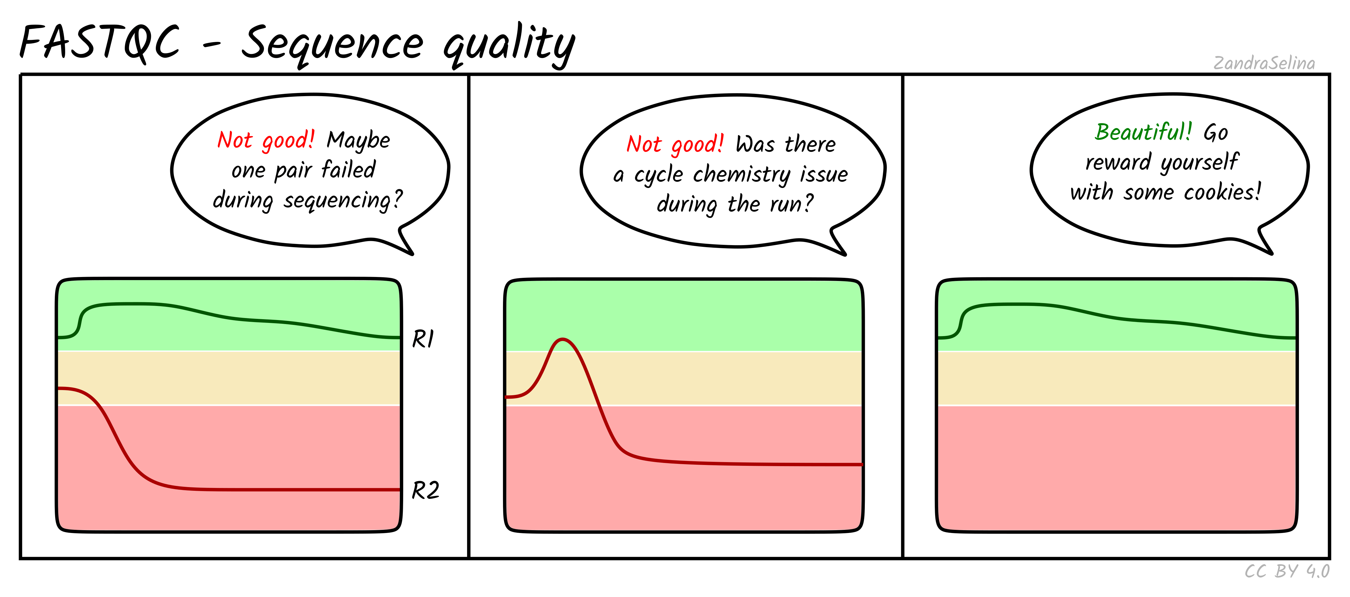
Per base sequence quality
Shows the distribution of quality scores at each position across all reads. You want high and stable quality across the read. A small quality drop at the end of R2 is common and usually not a problem.
Per tile sequence quality
Reports whether specific regions of the flowcell produced lower quality reads. Uneven tiles can indicate instrument issues or bubble formation, but this module rarely shows problems in modern Illumina data.
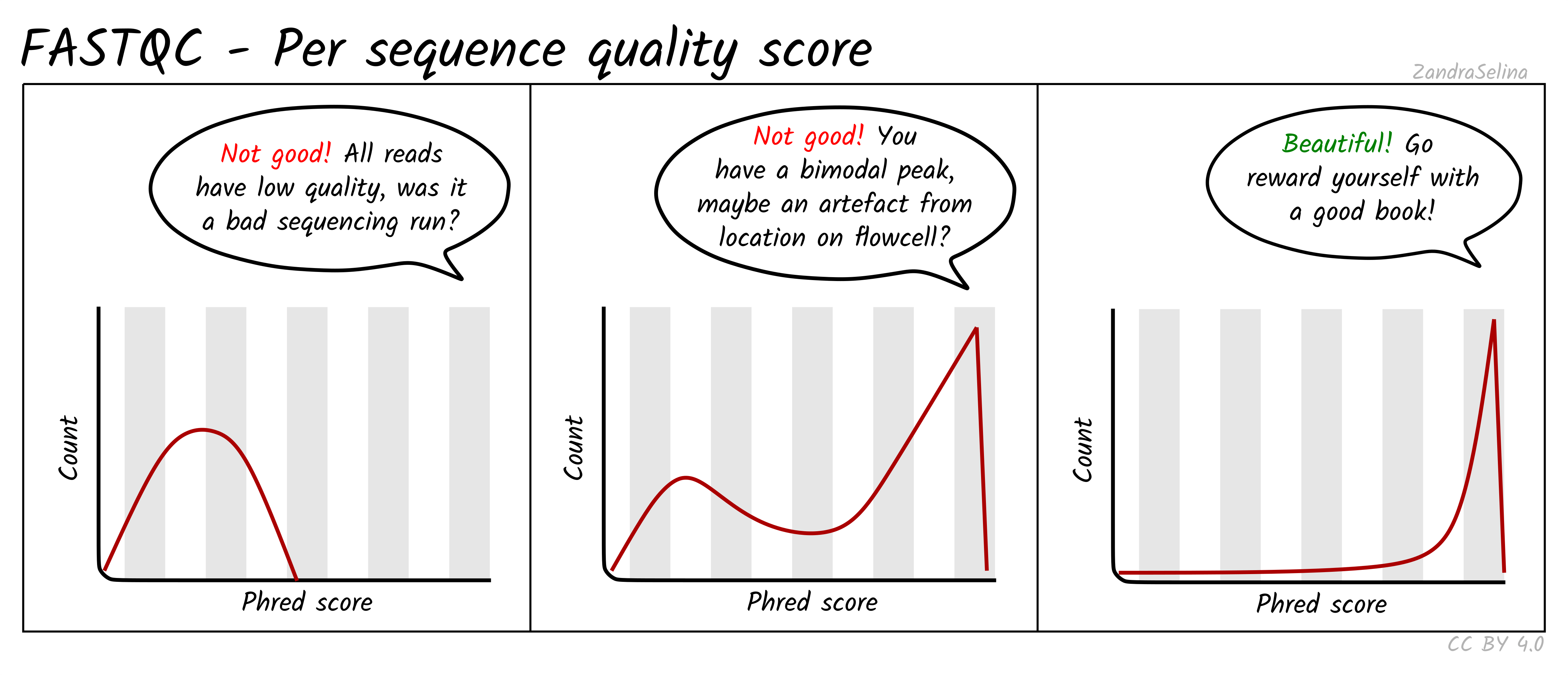
Per sequence quality scores
Shows how many reads have high or low overall quality. A good dataset has most reads with high scores and very few reads with low quality.
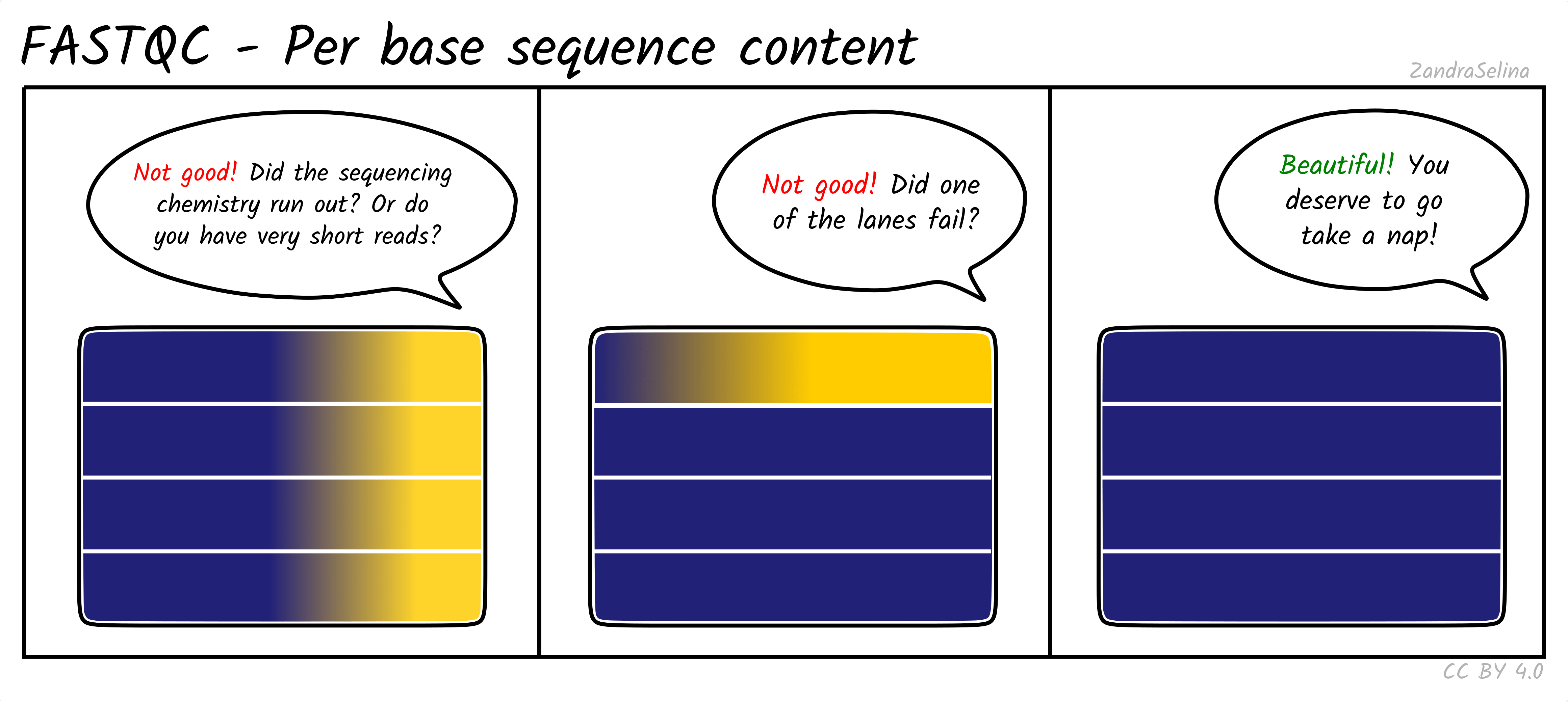
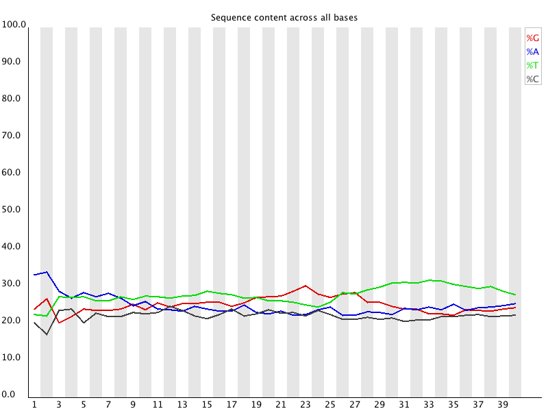
Per base sequence content
Shows the proportion of A, C, G, and T at each cycle. For genomic resequencing, all four lines should be close to 25 percent. RNA-seq usually shows imbalanced composition in early cycles due to biased priming and transcript composition. Mild imbalance at the start of the read is normal and does not require trimming.
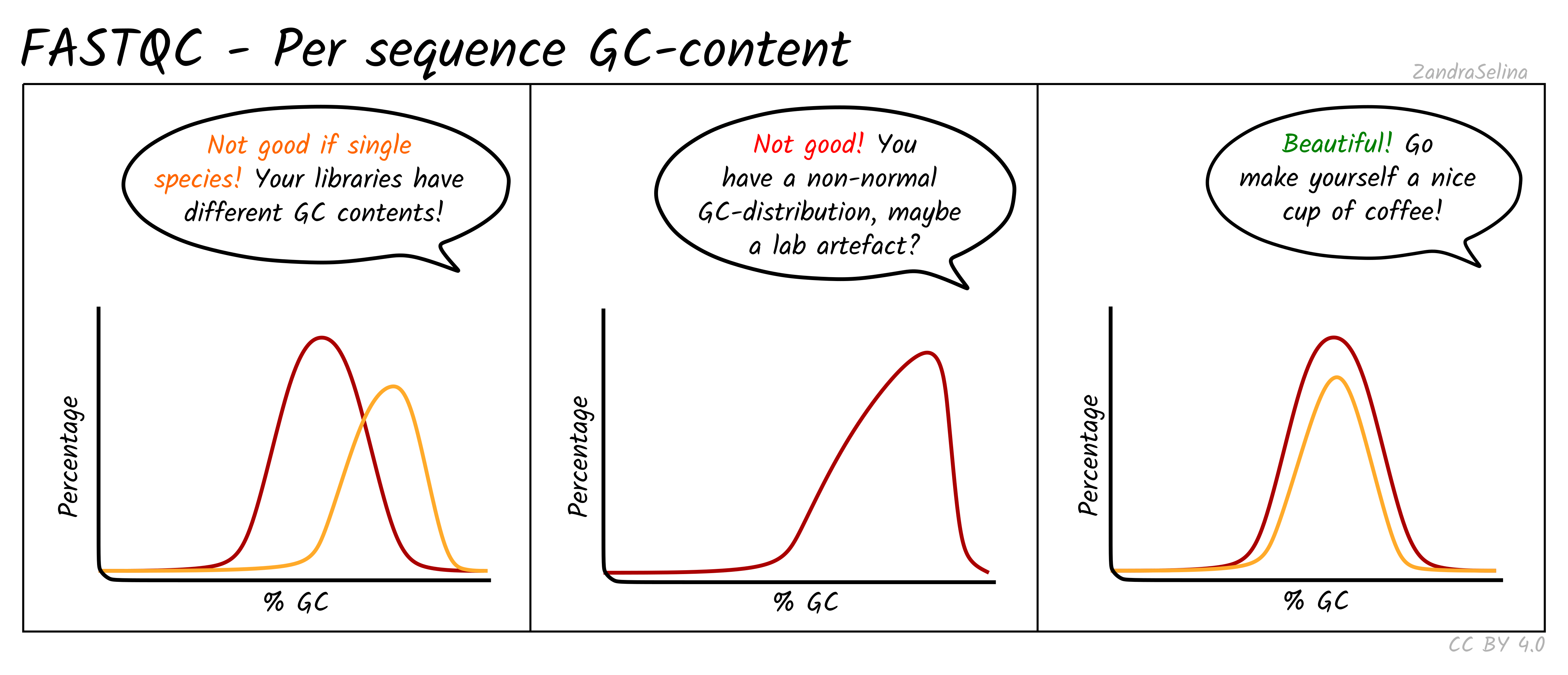
Per sequence GC content
Shows the GC distribution across all reads. RNA-seq often fails this test because expressed transcripts are not GC neutral. Only pronounced multi-modal or extremely shifted distributions are concerning, for example when contamination from another organism is suspected.
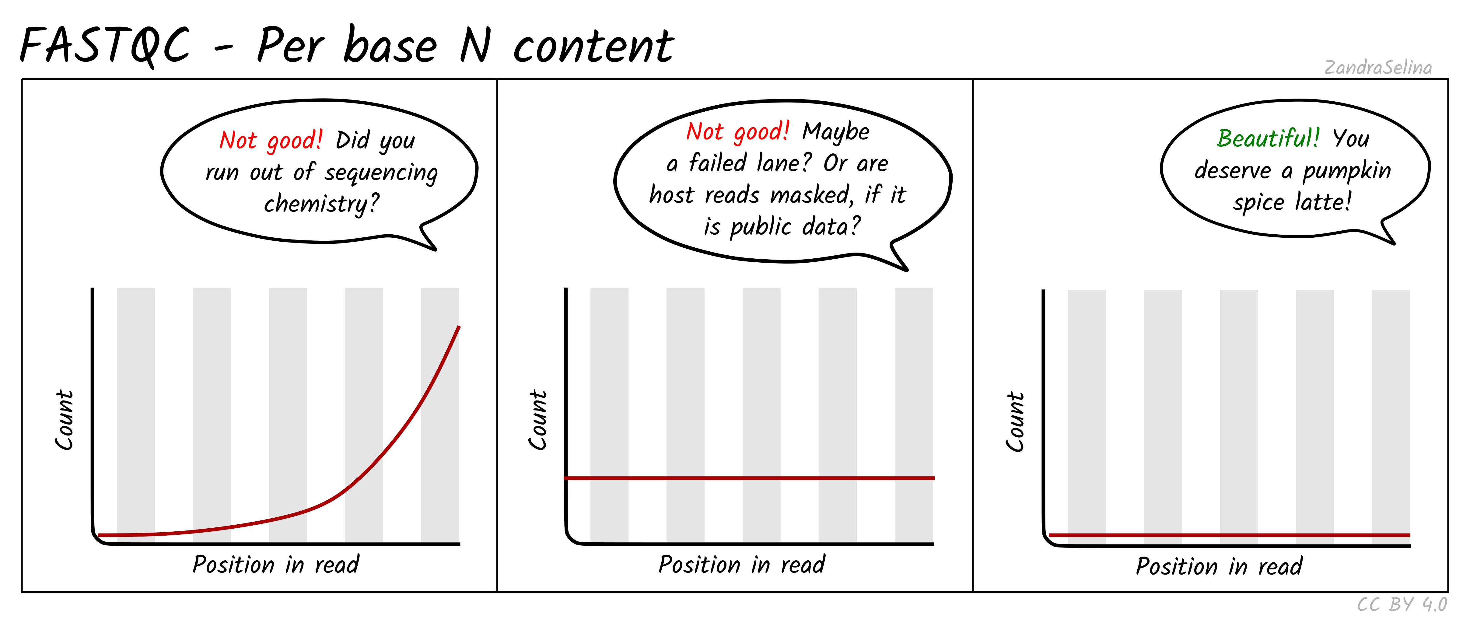
Per base N content
Reports the percentage of unidentified bases (N) at each position. This should be near zero for modern Illumina runs. High N content indicates failed cycles or poor sequencing chemistry.
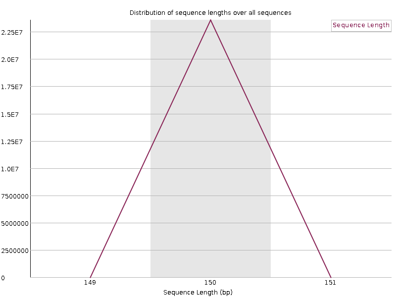
Sequence length distribution
Shows the distribution of read lengths. Standard RNA-seq libraries should have a narrow peak at the expected read length. Variable lengths usually appear after trimming or for specialized protocols such as small RNA.
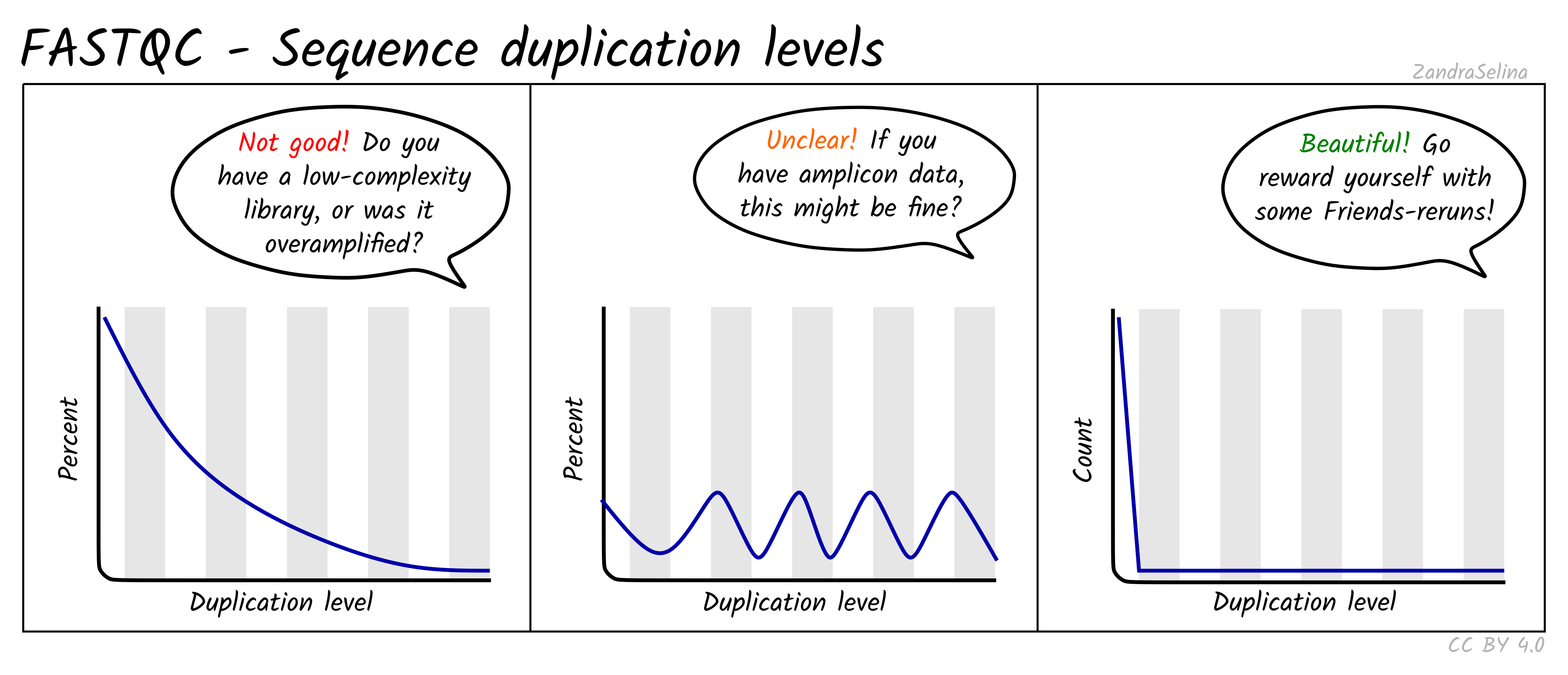
Sequence duplication levels
Reports how many reads are exact duplicates. Some duplication is normal in RNA-seq because highly expressed genes produce many identical fragments. Very high duplication, especially combined with low library size, can indicate low library complexity or overamplification.
Overrepresented sequences
Lists specific sequences that occur more often than expected. Common sources include ribosomal RNA fragments, poly A tails, adapter sequence, or reads from highly expressed transcripts. Some overrepresented sequences are expected, but very high levels may indicate contamination or poor rRNA depletion.
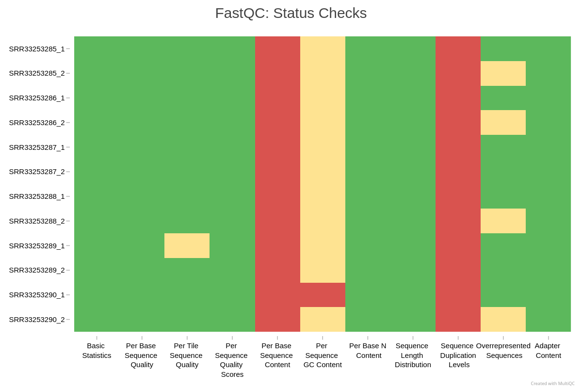
Aggregating reports with MultiQC
FastQC generates a separate HTML file per sample. MultiQC consolidates all reports and allows easy comparison of replicates.
Trimming adapter sequences
Before deciding whether to trim reads, it is essential to understand what adapters are and why they appear in sequencing data.
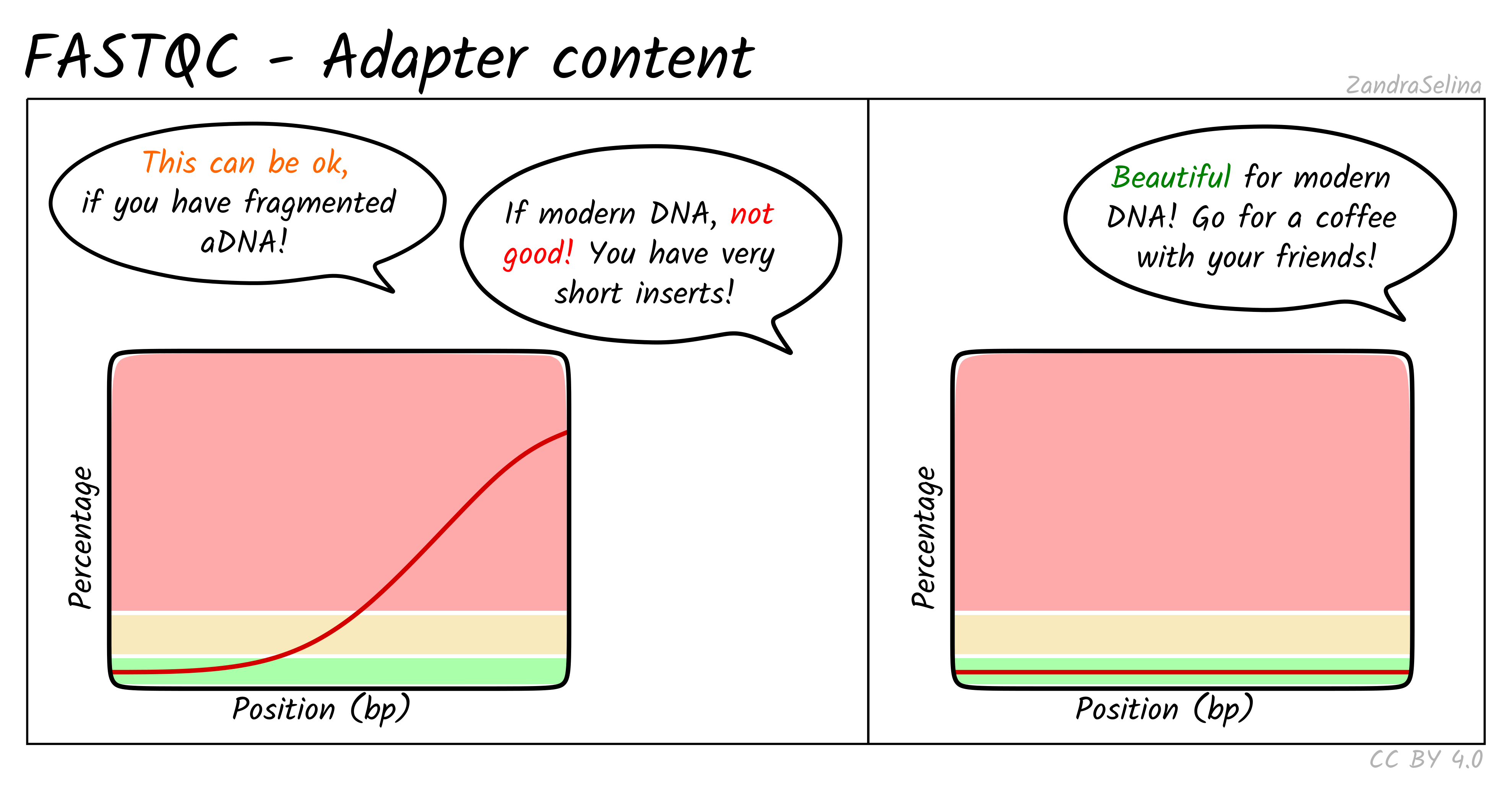
Adapters are short synthetic DNA sequences ligated to both ends of each fragment during library preparation. They provide primer binding sites needed for cluster amplification and sequencing. Ideally, the sequenced fragment is long enough that the machine reads only biological DNA. However, when the insert is shorter than the read length, the sequencer runs into the adapter sequence, which produces adapter contamination at the ends of reads.
Many users assume that adapters must always be trimmed, but this is not true for typical RNA-seq workflows.
Do we need to trim reads for standard RNA-seq workflows?
For alignment based RNA-seq, adapter trimming is usually not required. Modern aligners such as HISAT2 and STAR detect and soft clip adapter sequence automatically. Soft-clipped bases do not contribute to mismatches or mapping penalties, so adapters generally do not harm alignment quality.
In contrast, unnecessary trimming can introduce new problems:
- shorter reads and lower mapping power
- uneven trimming across samples and artificial differences
- reduction in read complexity
- broken read pairing for paired-end sequencing
- more parameters to track for reproducibility
Trimming is recommended only in specific situations:
- very short inserts, for example degraded RNA or ancient DNA
- adapter sequence dominating read tails, for example more than 10-15 percent adapter content
- transcript assembly workflows such as StringTie or Scallop, which benefit from uniform read lengths
- small RNA or miRNA libraries, where inserts are intentionally very short and adapter presence is guaranteed
Exercise: evaluate the QC results
Inspect your MultiQC report
Using the MultiQC HTML report, answer:
- Do all replicates show similar per base sequence quality profiles?
- Is adapter content high enough to impact analysis?
- Is any sample behaving differently from the rest, for example in number of reads, quality, duplication, or GC percentage?
Typical interpretation for this dataset (students should compare with their own):
- All replicates show high, stable sequence quality.
- Adapter signal appears only at the extreme ends of reads for selected samples and is less than 4 percent.
- No samples show concerning patterns or biases.
- Trimming is therefore unnecessary for this dataset.
Optional reference: how to trim adapters with fastp
(not part of the hands-on)
Sometimes you may encounter datasets where trimming is appropriate, for example short inserts, small RNA, or visibly high adapter content in QC. Although we will not trim reads in this workshop, here is a minimal example you can use in your own projects if trimming becomes necessary.
fastp is a fast, widely used tool that can automatically
detect adapters, trim them, filter low quality reads, and generate QC
reports.
Summary
- FastQC and MultiQC provide essential diagnostics for RNA-seq data.
- Some FastQC warnings are normal for RNA-seq and do not indicate problems.
- Aligners soft clip adapters, so trimming is usually unnecessary for alignment based RNA-seq.
- QC helps detect outliers before alignment and quantification.
Content from A. Genome-based quantification (STAR + featureCounts)
Last updated on 2026-06-16 | Edit this page
Estimated time: 70 minutes
Overview
Questions
- How do we map RNA-seq reads to a reference genome?
- How do we determine library strandness before alignment?
- How do we quantify reads per gene using featureCounts?
- How do we submit mapping jobs on RCAC clusters with SLURM?
Objectives
- Check RNA-seq library strandness using Salmon.
- Index a reference genome for STAR.
- Map reads to the genome using STAR.
- Quantify gene level counts with featureCounts.
- Interpret basic alignment and counting statistics.
Introduction
In this episode we move from raw FASTQ files to genome based gene
counts.
This workflow has three major steps:
- Determine library strandness: STAR does not infer strandness
automatically.
featureCountsrequires the correct setting. - Map reads to the genome using STAR: STAR is a splice aware aligner designed for RNA-seq data.
- Count mapped reads per gene using
featureCounts
This represents one of the two standard quantification strategies in
RNA-seq.
The alternative method (B. transcript based quantification with Salmon
or Kallisto) will be covered in Episode 4B.
Step 1: Checking RNA-seq library strandness
Why strandness matters
RNA-seq libraries can be:
- unstranded
- stranded forward
- stranded reverse
Stranded protocols are common in modern kits, but old GEO and SRA
datasets are often unstranded.
featureCounts must be given the correct strand setting. If the wrong
setting is used, most reads will be counted against incorrect genes.
STAR does not infer strandness automatically, so we must determine it before alignment.
Detecting strandness with Salmon
Salmon can infer strandness directly from raw FASTQ files without any
alignment.
We run Salmon with -l A, which tells it to explore all
library types.
BASH
sinteractive -A rcac-workshop -q standby -p cpu -N 1 -n 4 --time=1:00:00

cd $SCRATCH/rnaseq-workshop
mkdir -p results/strand_check

module load biocontainers
module load salmon

salmon index --transcripts data/gencode.vM38.transcripts-clean.fa \
             --index data/salmon_index \
             --threads 4

salmon quant --index data/salmon_index \
             --libType A \
             --mates1 data/WT_Bcell_mock_rep1_R1.fastq.gz \
             --mates2 data/WT_Bcell_mock_rep1_R2.fastq.gz \
             --output results/strand_check \
             --threads 4
The important output is in
results/strand_check/lib_format_counts.json:
JSON
{
    "read_files": "[ data/WT_Bcell_mock_rep1_R1.fastq.gz, data/WT_Bcell_mock_rep1_R2.fastq.gz]",
    "expected_format": "IU",
    "compatible_fragment_ratio": 1.0,
    "num_compatible_fragments": 11994681,
    "num_assigned_fragments": 11994681,
    "num_frags_with_concordant_consistent_mappings": 10472924,
    "num_frags_with_inconsistent_or_orphan_mappings": 2280227,
    "strand_mapping_bias": 0.5082214861866657,
    "MSF": 0,
    "OSF": 0,
    "ISF": 5322565,
    "MSR": 0,
    "OSR": 0,
    "ISR": 5150359,
    "SF": 1149290,
    "SR": 1130937,
    "MU": 0,
    "OU": 0,
    "IU": 0,
    "U": 0
}
Interpreting
lib_format_counts.jsonThis JSON file reports Salmon’s automatic library type detection.
"expected_format": "IU": This is Salmon’s conclusion. “I” means Inward (correct for paired-end reads) and “U” means Unstranded."strand_mapping_bias": 0.508: This is the key evidence. A value near 0.5 (50%) indicates that reads mapped equally to both the sense and antisense strands, the definitive sign of an unstranded library."ISF"and"ISR": These are the counts for Inward-Sense-Forward (36.4M) and Inward-Sense-Reverse (35.2M) fragments. Because these values are almost equal, they confirm the ~50/50 split seen in the strand bias.
Common results:
| Code | Meaning |
|---|---|
| IU | unstranded |
| ISR | stranded reverse (paired end) |
| ISF | stranded forward (paired end) |
| SR | stranded reverse (single end) |
| SF | stranded forward (single end) |
Conclusion: The data is unstranded. We will record this and supply it to STAR/featureCounts.
Step 2: Preparing the reference genome for alignment
STAR requires a genome index. Indexing builds a searchable data structure that speeds up alignment.
Required input:
- genome FASTA file
- annotation file (GTF or GFF3)
- output directory for the index
Optionally, annotation improves splice junction detection and yields better alignments.
Why STAR?
- Splice-aware
- Extremely fast
- Produces high-quality alignments
- Well supported and widely used
- Compatible with downstream tools such as featureCounts, StringTie, and RSEM
Optional alternatives include HISAT2 and Bowtie2, but STAR remains the standard for high-depth Illumina RNA-seq.
Exercise: Read the STAR manual
Check the “Generating genome indexes” section of
the
STAR
manual
Which options are required for indexing?
Key options:
-
--runMode genomeGenerate
-
--genomeDirdirectory to store the index
-
--genomeFastaFilesthe FASTA file
-
--sjdbGTFfileannotation (recommended)
-
--runThreadNnumber of threads
-
--sjdbOverhangread length minus one (100 is a safe default)
Indexing the Genome with STAR
Below is a minimal SLURM job script for building the STAR genome
index. Create a file named index_genome.sh in
$SCRATCH/rcac_rnaseq/scripts with this content:
BASH
#!/bin/bash
#SBATCH --nodes=1
#SBATCH --ntasks=1
#SBATCH --cpus-per-task=20
#SBATCH --account=rcac-rnaseq
#SBATCH --qos=standby
#SBATCH --partition=cpu
#SBATCH --time=1:00:00
#SBATCH --job-name=star_index
#SBATCH --output=cluster-%x.%j.out
#SBATCH --error=cluster-%x.%j.err

module load biocontainers
module load star

data_dir="${SCRATCH}/rnaseq-workshop/data"
genome="${data_dir}/GRCm39.primary_assembly.genome.fa"
gtf="${data_dir}/gencode.vM38.primary_assembly.basic.annotation.gtf"
indexdir="${data_dir}/star_index"

STAR \
    --runMode genomeGenerate \
    --runThreadN ${SLURM_CPUS_ON_NODE} \
    --genomeDir ${indexdir} \
    --genomeFastaFiles ${genome} \
    --sjdbGTFfile ${gtf}
Submit the job:
Indexing requires about 30 to 45 minutes.
The index directory is now ready for use in mapping and should have
contents like this: Location: $SCRATCH/rcac_rnaseq/data
Contents of star_index/:
BASH
star_index/
├── chrLength.txt
├── chrNameLength.txt
├── chrName.txt
├── chrStart.txt
├── exonGeTrInfo.tab
├── exonInfo.tab
├── geneInfo.tab
├── Genome
├── genomeParameters.txt
├── Log.out
├── SA
├── SAindex
├── sjdbInfo.txt
├── sjdbList.fromGTF.out.tab
├── sjdbList.out.tab
└── transcriptInfo.tabDo I need the GTF for indexing?
No, but it is strongly recommended.
Including it improves splice junction detection and increases mapping
accuracy.
Step 3: Mapping reads with STAR
Once the genome index is ready, we can align reads.
For aligning reads, important STAR options are:
--runThreadN--genomeDir--readFilesIn-
--readFilesCommand zcatfor gzipped FASTQ files --outSAMtype BAM SortedByCoordinate--outSAMunmapped Within
STAR’s defaults are tuned for mammalian genomes. If working with plants, fungi, or repetitive genomes, additional tuning may be required.
Exercise: Write a STAR alignment command
Write a basic STAR alignment command using your genome index and paired FASTQ files.
Mapping many FASTQ files with a SLURM array
When having multiple samples, array jobs simplify submission.
First, we will create samples.txt file with just the
sample names
BASH
cd $SCRATCH/rnaseq-workshop/data
ls *_R1.fastq.gz | sed 's/_R1.fastq.gz//' > ${SCRATCH}/rnaseq-workshop/scripts/samples.txt
BASH
#!/bin/bash
#SBATCH --nodes=1
#SBATCH --ntasks=1
#SBATCH --cpus-per-task=20
#SBATCH --account=rcac-rnaseq
#SBATCH --qos=standby
#SBATCH --partition=cpu
#SBATCH --time=8:00:00
#SBATCH --job-name=read_mapping
#SBATCH --array=1-8
#SBATCH --output=cluster-%x.%j.out
#SBATCH --error=cluster-%x.%j.err

module load biocontainers
module load star

FASTQ_DIR="$SCRATCH/rnaseq-workshop/data"
GENOME_INDEX="$SCRATCH/rnaseq-workshop/data/star_index"
OUTDIR="$SCRATCH/rnaseq-workshop/results/mapping"

mkdir -p $OUTDIR

SAMPLE=$(sed -n "${SLURM_ARRAY_TASK_ID}p" samples.txt)

R1=${FASTQ_DIR}/${SAMPLE}_R1.fastq.gz
R2=${FASTQ_DIR}/${SAMPLE}_R2.fastq.gz

STAR \
    --runThreadN ${SLURM_CPUS_ON_NODE} \
    --genomeDir $GENOME_INDEX \
    --readFilesIn $R1 $R2 \
    --readFilesCommand zcat \
    --outFileNamePrefix $OUTDIR/$SAMPLE \
    --outSAMunmapped Within \
    --outSAMtype BAM SortedByCoordinate
Submit:
Why use an array job?
Think about this:
- We have eight samples, each with two FASTQ files
- Having eight separate slurm jobs means:
- Copy-pasting the same command eight times
- Higher chance of typos or mistakes
- if mapping with single slurm file, sequential execution = slower
- Samples can run independently
Why is a job array a good choice?
Arrays allow us to run identical commands across many inputs:
- All samples are processed the same way
- Runs in parallel
- Simplifies submission
- Reduces copy-paste errors
- Minimizes runtime cost on the cluster
Step 4: Assessing alignment quality
STAR produces several useful files, particularly:
Log.final.out
Contains mapping statistics, including % uniquely mapped.Aligned.sortedByCoord.out.bam
Ready for downstream quantification.
To summarize alignment statistics across samples, we use MultiQC:
BASH
cd $SCRATCH/rnaseq-workshop
module load biocontainers
module load multiqc

multiqc results/mapping -o results/qc_alignment
Key metrics to review
-
Uniquely mapped reads — typically 60–90% is
good
-
Multi-mapped reads — depends on genome, but >20%
is concerning
-
Unmapped reads — check reasons (mismatches? too
short?)
- Mismatch rate — high values indicate quality or contamination issues
Exercise: Examine your alignment metrics
Using your MultiQC alignment report:
- Which sample has the highest uniquely mapped percentage?
- Are any samples clear outliers?
- Does mapped/unmapped reads appear consistent across samples?
Example interpretation for this dataset:
- All samples have ~80% uniquely mapped reads.
- No sample is an outlier.
- mapped/unmapped reads consistent across samples
Step 5: Quantifying gene counts with featureCounts
Once the reads have been aligned and sorted, we can quantify how many
read pairs map to each gene. This gives us gene-level counts that we
will later use for differential expression. For alignment-based RNA-seq
workflows, featureCounts is the recommended tool because it
is fast, robust, and compatible with most gene annotation formats.
featureCounts uses two inputs:
- A set of aligned BAM files (sorted by coordinate)
- A GTF annotation file describing gene models
It assigns each read (or read pair) to a gene based on the exon boundaries.
Important: stranded or unstranded?
featureCounts needs to know whether your dataset is
stranded.
-
-s 0unstranded -
-s 1stranded forward -
-s 2stranded reverse
From our Salmon strandness check, this dataset behaves as
unstranded, so we will use -s 0.
Running featureCounts
We will create a new directory for count output:
Below is an example SLURM script to count all BAM files at once.
BASH
#!/bin/bash
#SBATCH --nodes=1
#SBATCH --ntasks=1
#SBATCH --cpus-per-task=16
#SBATCH --account=rcac-rnaseq
#SBATCH --qos=standby
#SBATCH --partition=cpu
#SBATCH --time=1:00:00
#SBATCH --job-name=featurecounts
#SBATCH --output=cluster-%x.%j.out
#SBATCH --error=cluster-%x.%j.err

module load biocontainers
module load subread

GTF="$SCRATCH/rnaseq-workshop/data/gencode.vM38.primary_assembly.basic.annotation.gtf"
BAMS="$SCRATCH/rnaseq-workshop/results/mapping/*.bam"
output_dir="$SCRATCH/rnaseq-workshop/results/counts"

featureCounts \
  -T ${SLURM_CPUS_PER_TASK} \
  -p \
  -s 0 \
  -t exon \
  -g gene_id \
  -a ${GTF} \
  -o ${output_dir}/gene_counts.txt \
  ${BAMS}
Submit the job:
gene_counts.txt will contain:
- one row per gene
- one column per sample
Step 6: QC on counts
Before proceeding to differential expression, it is good practice to perform some QC on the count data. We can again use MultiQC to summarize featureCounts statistics:
BASH
cd $SCRATCH/rnaseq-workshop
mkdir -p results/qc_counts
module load biocontainers
module load multiqc
multiqc results/counts -o results/qc_countsExercise: Examine your counting metrics
Using your MultiQC featureCounts report:
- Which sample has the lowest percent assigned, and what are common reasons for lower assignment?
- Which unassigned category is the largest, and what does it indicate?
- Does the sample with the most assigned reads also have the highest percent assigned?
- What does “Unassigned: No Features” mean, and why might it occur?
- Are multi-mapped reads a concern for RNA-seq differential expression?
Example interpretation for this dataset:
- The sample with the lowest assignment rate may vary. Causes include low complexity, incomplete annotation, or more intronic reads.
- Unmapped or No Features dominate. These reflect reads that do not align or do not overlap annotated exons.
- No. Total assigned reads depend on depth, while percent assigned reflects library quality.
- Reads mapped outside annotated exons, often from intronic regions, unannotated transcripts, or incomplete annotation.
- Multi-mapping is expected for paralogs and repeats. It is usually fine as long as the rate is consistent across samples.
Summary
- STAR is a fast splice-aware aligner widely used for RNA-seq.
- Genome indexing requires FASTA and optionally GTF for improved splice detection.
- Mapping is efficiently performed using SLURM array jobs.
- Alignment statistics (from
Log.final.out+ MultiQC) must be reviewed. - Strandness should be inferred using aligned BAM files.
- Final BAM files are ready for downstream counting.
-
featureCountsis used to obtain gene-level counts for differential expression. - Exons are counted and summed per gene.
- The output is a simple matrix for downstream statistical analysis.
Content from B. Transcript-based quantification (Kallisto)
Last updated on 2026-06-16 | Edit this page
Estimated time: 70 minutes
Overview
Questions
- How do we quantify expression without genome alignment?
- What inputs does Kallisto require?
- How do we run Kallisto for paired-end RNA-seq data?
- How do we interpret transcript-level outputs (TPM, est_counts)?
- How do we summarize transcripts to gene-level counts using tximport?
Objectives
- Build a transcriptome index for Kallisto.
- Quantify transcript abundance directly from FASTQ files.
- Understand key Kallisto output files.
- Summarize transcript-level estimates to gene-level counts.
- Prepare counts for downstream differential expression.
Introduction
In the previous episode, we mapped reads to the genome using STAR and generated gene-level counts with featureCounts.
In this episode, we use an alternative quantification strategy:
- Build a transcriptome index
- Quantify expression directly from FASTQ files using Kallisto (without alignment)
- Summarize transcript estimates back to gene-level counts
This workflow is faster, uses less storage, and models transcript-level uncertainty.
Why Kallisto?
Kallisto uses pseudo-alignment to rapidly quantify transcript abundances without traditional read mapping. Key advantages include:
- Speed: Kallisto is extremely fast, typically completing in 2-3 minutes per sample.
- Accuracy: Comparable accuracy to alignment-based methods for quantification.
- Bootstrap support: Native support for uncertainty estimation via bootstraps (useful for sleuth).
- Low resource usage: No large BAM files generated, minimal storage requirements.
Kallisto is ideal when you do not need alignment files, want fast quantification, or plan to use sleuth for differential transcript analysis.
When should I use transcript-based quantification?
Kallisto is ideal when:
- You do not need alignment files.
- You want transcript-level TPMs.
- You want fast quantification.
- Storage is limited (no BAM files generated).
- You plan to use sleuth for differential transcript expression.
It is not ideal if you need splice junctions, variant calling, or visualization in IGV (all those depend on alignment files).
Step 1: Preparing the transcriptome reference
Kallisto requires a transcriptome FASTA file (all
annotated transcripts). We previously downloaded the transcripts file
from GENCODE for this purpose
(gencode.vM38.transcripts-clean.fa).
Why transcriptome choice matters
Transcript-level quantification inherits all assumptions of the annotation. Missing or incorrect transcripts → biased TPM estimates.
Building the Kallisto index
The Kallisto index is lightweight and quick to build:
BASH
cd $SCRATCH/rnaseq-workshop
mkdir -p data/kallisto_index

module load biocontainers
module load kallisto

kallisto index \
    -i data/kallisto_index/transcripts.idx \
    data/gencode.vM38.transcripts-clean.fa
This creates an index file that Kallisto uses for pseudo-alignment. Index building typically takes 2-3 minutes for a mammalian transcriptome.
Kallisto vs Salmon index
Note that Kallisto and Salmon indices are not interchangeable. Each tool has its own index format:
- Kallisto: Single
.idxfile - Salmon: Directory with multiple files
You must build a separate index for each tool.
Step 2: Quantifying transcript abundances
The core Kallisto command is kallisto quant. We use the
transcript index and paired-end FASTQ files.
Example command:
BASH
kallisto quant \
    -i data/kallisto_index/transcripts.idx \
    -o results/kallisto_quant/WT_Bcell_mock_rep1 \
    -b 100 \
    -t 16 \
    data/WT_Bcell_mock_rep1_R1.fastq.gz \
    data/WT_Bcell_mock_rep1_R2.fastq.gz
Important flags:
-
-i→ path to the Kallisto index -
-o→ output directory for this sample -
-b 100→ number of bootstrap samples (useful for uncertainty estimation and sleuth) -
-t 16→ number of threads to use
Strand-specific libraries
For strand-specific libraries, add the appropriate flag:
-
--rf-strandedfor reverse-stranded libraries (e.g., Illumina TruSeq stranded) -
--fr-strandedfor forward-stranded libraries
Our dataset is unstranded (detected as
IU in Step 0), so we omit these flags.
Bootstrap samples
The -b 100 flag generates 100 bootstrap samples. These
are useful for:
- Estimating uncertainty in transcript abundance
- Required if you plan to use sleuth for differential expression
- Can be omitted if you only use DESeq2/edgeR (for faster runtime)
For DESeq2 analysis only, you can use -b 0 or omit the
flag entirely.
Step 3: Running Kallisto for many samples
We use a SLURM array job for efficiency and consistency.
First, create a sample list (or reuse the one from Episode 4A):
BASH
cd $SCRATCH/rnaseq-workshop/data
ls *_R1.fastq.gz | sed 's/_R1.fastq.gz//' > $SCRATCH/rnaseq-workshop/scripts/samples.txt
Array job:
BASH
#!/bin/bash
#SBATCH --nodes=1
#SBATCH --ntasks=1
#SBATCH --cpus-per-task=16
#SBATCH --account=rcac-rnaseq
#SBATCH --qos=standby
#SBATCH --partition=cpu
#SBATCH --time=1:00:00
#SBATCH --job-name=kallisto_quant
#SBATCH --array=1-8
#SBATCH --output=cluster-%x.%j.out
#SBATCH --error=cluster-%x.%j.err

module load biocontainers
module load kallisto

DATA="$SCRATCH/rnaseq-workshop/data"
INDEX="$SCRATCH/rnaseq-workshop/data/kallisto_index/transcripts.idx"
OUT="$SCRATCH/rnaseq-workshop/results/kallisto_quant"

SAMPLE=$(sed -n "${SLURM_ARRAY_TASK_ID}p" samples.txt)

mkdir -p ${OUT}/${SAMPLE}

R1=${DATA}/${SAMPLE}_R1.fastq.gz
R2=${DATA}/${SAMPLE}_R2.fastq.gz

kallisto quant \
    -i $INDEX \
    -o $OUT/$SAMPLE \
    -b 100 \
    -t ${SLURM_CPUS_ON_NODE} \
    $R1 $R2 &> $OUT/$SAMPLE/${SAMPLE}.log
Submit:
The typical run time is ~2-3 minutes per sample (faster than Salmon).
Why use an array job here?
Kallisto runs very quickly and produces small output. The advantage of array jobs is consistency: all samples are quantified with identical parameters and metadata. This ensures that transcript-level TPM and count estimates are directly comparable across samples.
Inspect results
After Kallisto finishes, each sample directory contains a small set of output files:
WT_Bcell_mock_rep1/
├── abundance.tsv          # IMPORTANT: transcript-level TPM, counts, effective lengths
├── abundance.h5           # IMPORTANT: HDF5 format with bootstrap data (for sleuth)
└── run_info.json          # IMPORTANT: run parameters and mapping statistics
What is inside abundance.tsv?
This file contains the transcript-level quantification results:
- target_id: transcript ID
- length: transcript length
- eff_length: effective length adjusted for fragment distribution
- est_counts: estimated number of reads assigned to that transcript
- tpm: within-sample normalized abundance (Transcripts Per Million)
Example:
target_id                  length  eff_length  est_counts  tpm
ENSMUST00000193812.2       1070    775.000     0.000       0.000000
ENSMUST00000082908.3       110     110.000     0.000       0.000000
ENSMUST00000162897.2       4153    3483.630    1.000       0.013994
ENSMUST00000159265.2       2989    2694.000    0.000       0.000000
ENSMUST00000070533.5       3634    3339.000    0.000       0.000000
Key QC metrics to review
Open run_info.json and check:
- n_processed: total number of reads processed
- n_pseudoaligned: number of reads that pseudoaligned to transcripts
- p_pseudoaligned: proportion of reads pseudoaligned (mapping rate)
These metrics provide a first-pass sanity check before summarizing the results to gene-level counts.
What does Kallisto count?
est_counts is a model-based estimate, not raw counts of
reads. TPM values are within-sample normalized and should not
be directly compared across samples for statistical testing.
Step 4: Summarizing to gene-level counts
(tximport)
Most differential expression tools (DESeq2, edgeR) require gene-level counts. We convert transcript estimates → gene-level matrix.
Prepare tx2gene mapping
We need a mapping file that links transcript IDs to gene IDs. The GTF annotation file contains this information.
BASH
cd $SCRATCH/rnaseq-workshop/data
awk -F'\t' '$3=="transcript" {
    match($9, /transcript_id "([^"]+)"/, tx);
    match($9, /gene_id "([^"]+)"/, gene);
    print tx[1] "\t" gene[1]
}' gencode.vM38.primary_assembly.basic.annotation.gtf > tx2gene.tsv
Next, we process this mapping in R. Load the modules and start the R session:
In the R session, read in the tx2gene mapping and run
tximport:
R
setwd(paste0(Sys.getenv("SCRATCH"), "/rnaseq-workshop"))
library(readr)
library(tximport)

tx2gene <- read_tsv("data/tx2gene.tsv", col_types = "cc", col_names = FALSE)
samples <- read_tsv("scripts/samples.txt", col_names = FALSE)
files <- file.path("results/kallisto_quant", samples$X1, "abundance.h5")
names(files) <- samples$X1

txi <- tximport(files,
                type = "kallisto",
                tx2gene = tx2gene)
saveRDS(txi, file = "results/kallisto_quant/txi.rds")
txi$counts now contains gene-level counts suitable for
DESeq2.
R
> head(txi$counts)
                      WT_Bcell_mock_rep1 WT_Bcell_mock_rep2 WT_Bcell_mock_rep3 WT_Bcell_mock_rep4
ENSMUSG00000000001.5          473.4426         553.7849         826.9969         676.9101
ENSMUSG00000000003.16           0.0000           0.0000           0.0000           0.0000
ENSMUSG00000000028.16          40.5783          33.9665          55.3055          97.8451
ENSMUSG00000000031.20           0.0000           0.0000           0.0000           0.0000
ENSMUSG00000000037.18          19.2220           9.5997          16.9515          20.2265
ENSMUSG00000000049.12           0.0000           5.0221           1.9846           1.0164
                      WT_Bcell_IR_rep1 WT_Bcell_IR_rep2 WT_Bcell_IR_rep3 WT_Bcell_IR_rep4
ENSMUSG00000000001.5        724.1176        813.8484        689.2341        752.1567
ENSMUSG00000000003.16         0.0000          0.0000          0.0000          0.0000
ENSMUSG00000000028.16        41.6915         63.8123         48.3421         55.7892
ENSMUSG00000000031.20         0.0000          0.0000          0.0000          0.0000
ENSMUSG00000000037.18        19.6807         18.9451         22.3456         17.8923
ENSMUSG00000000049.12 0.9937 9.1869 2.3456 4.5678Why use the default countsFromAbundance setting?
We use the default countsFromAbundance = "no" because
DESeqDataSetFromTximport() (used in Episode 05b)
automatically incorporates the txi$length matrix to correct
for transcript length bias.
Using "lengthScaledTPM" would apply length correction
twice—once in tximport and again in DESeq2—potentially introducing bias.
The default preserves Kallisto’s original estimated counts while letting
DESeq2 handle length normalization correctly.
Note: If you plan to use edgeR instead of DESeq2,
you may want countsFromAbundance = "lengthScaledTPM" since
edgeR’s DGEList doesn’t automatically use the length
matrix.
Using abundance.h5 vs abundance.tsv
tximport can read either format:
- abundance.h5: HDF5 format, includes bootstrap information, faster to read
- abundance.tsv: Plain text, easier to inspect manually
We use the .h5 files here because they load faster and
preserve bootstrap data for potential sleuth analysis. If you didn’t
generate bootstraps, you can use .tsv files instead.
Step 5: QC of quantification metrics
Use MultiQC to aggregate Kallisto results:
BASH
cd $SCRATCH/rnaseq-workshop
module load biocontainers
module load multiqc

multiqc results/kallisto_quant -o results/qc_kallisto
Inspect:
- pseudoalignment rates
- fragment length distributions
- consistency across samples
Exercise: examine your Kallisto outputs
Using your MultiQC summary and Kallisto outputs:
- What is the percent pseudoaligned for each sample, and are any samples outliers?
- Are the pseudoalignment rates consistent across samples?
- How similar are the fragment length distributions across samples?
- Check
run_info.jsonfor one sample - what parameters were used?
Example interpretation for this dataset:
- All samples show about 85 to 90 percent pseudoaligned. No sample is an outlier and the range is narrow.
- Pseudoalignment rates are consistent across all samples.
- Fragment length distributions should be nearly identical across samples.
- The
run_info.jsonshould show the index path, number of bootstraps, and thread count used.
Summary
- Kallisto performs fast, alignment-free transcript quantification.
- Salmon is used for strand detection before running Kallisto.
- A transcriptome FASTA is required for building the Kallisto index.
-
kallisto quantuses FASTQ files directly for pseudo-alignment. - Transcript-level outputs include TPM and estimated counts.
-
tximportconverts transcript estimates to gene-level counts withtype = "kallisto". - Gene-level counts from Kallisto are suitable for DESeq2.
Content from Gene-level QC and differential expression (DESeq2)
Last updated on 2026-06-16 | Edit this page
Estimated time: 85 minutes
Overview
Questions
- How do we explore RNA seq count data before running DESeq2.
- How do we restrict analysis to protein coding genes.
- How do we perform differential expression with DESeq2.
- How do we visualize sample relationships and DE genes.
- How do we save a useful DE results table with annotation and expression values.
Objectives
- Import count and sample metadata into R.
- Attach biotype and gene symbol annotation to Ensembl gene IDs.
- Explore library sizes, variance stabilizing transforms, distances, and PCA.
- Run DESeq2 for a two group comparison.
- Create a volcano plot with gene symbols.
- Export joined DE results including normalized counts and annotation.
Introduction
In this episode we move from count matrices to differential expression analysis and visualization.
The workflow has four parts:
- Import counts and sample metadata.
- Exploratory analysis on protein coding genes (quality checks).
- Differential expression analysis with DESeq2.
- Visualization and export of annotated DE results.
What you need for this episode
-
gene_counts_clean.txtgenerated from featureCounts
- a
samples.csvfile describing the experimental groups
- RStudio session on Scholar using Open OnDemand
While we created the count matrix in the previous episode, we still
need to create a sample metadata file. This file should contain at least
two columns: sample names matching the count matrix column names, and
the experimental condition (e.g., control vs treatment). Simply
copy/paste the following into a text file and save it in your
scripts directory as samples.csv:
sample,condition
WT_Bcell_mock_rep1,WT_mock
WT_Bcell_mock_rep2,WT_mock
WT_Bcell_mock_rep3,WT_mock
WT_Bcell_mock_rep4,WT_mock
WT_Bcell_IR_rep1,WT_IR
WT_Bcell_IR_rep2,WT_IR
WT_Bcell_IR_rep3,WT_IR
WT_Bcell_IR_rep4,WT_IR
Also, create a direcotry for DESeq2 results:
All analyses are performed in R through Open OnDemand
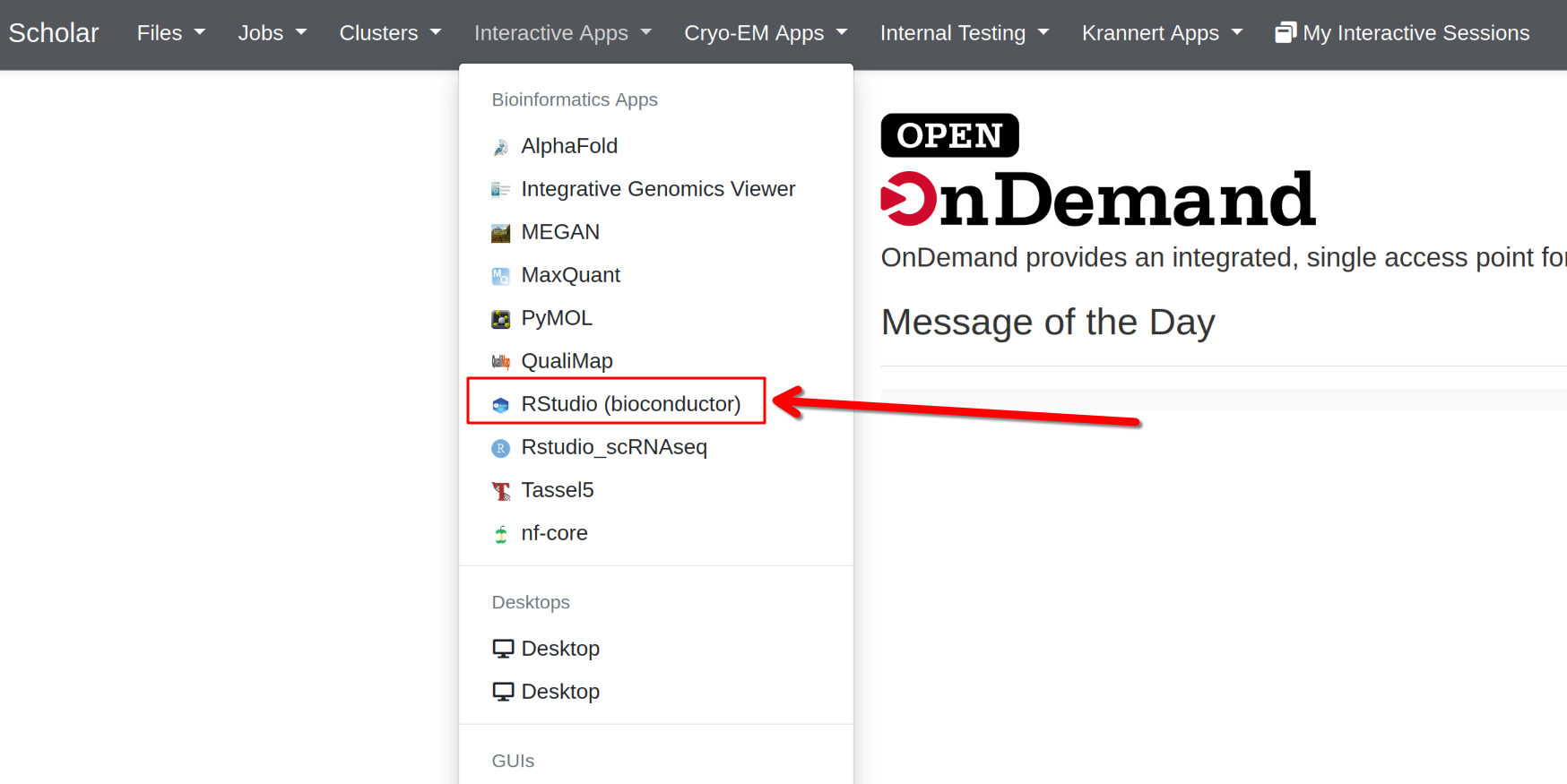
Step 1: Start Open OnDemand R session and prepare data
We will be using the OOD to start an interactive session on Scholar: https://gateway.negishi.rcac.purdue.edu
- Login using your Purdue credentials after clicking the above link
- Click on “Interactive Apps” in the top menu, and select “RStudio (Bioconductor)”
- Fill the job submission form as follows:
- queue:
rcac-rnaseq - Walltime:
4 - Number of cores:
4
- queue:
- Click “Launch” and wait for the RStudio session to start
- Once the session starts, you’ll will be able to click on “Connect to RStudio server” which will open the RStudio interface.
Once in RStudio, load the necessary libraries:
Setup: load packages and data
R
library(RColorBrewer)
library(EnsDb.Mmusculus.v79)
library(ensembldb)
library(tidyverse)
library(DESeq2)
library(ggplot2)
library(pheatmap)
library(readr)
library(dplyr)
library(ComplexHeatmap)
library(ggrepel)
library(vsn)
# Construct the path dynamically
work_dir <- file.path("/scratch/negishi", Sys.getenv("USER"), "rnaseq-workshop")
setwd(work_dir)

countsFile <- "results/counts/gene_counts_clean.txt"
# prepare this file first!
groupFile  <- "scripts/samples.csv"

coldata <-
  read.csv(
    groupFile,
    row.names = 1,
    header = TRUE,
    stringsAsFactors = TRUE
  )
coldata$condition <- as.factor(coldata$condition)

cts <- as.matrix(read.delim(countsFile, row.names = 1, header = TRUE))
We also load gene level annotation tables prepared earlier.
R
mart <-
  read.csv(
    "data/mart.tsv",
    sep = "\t",
    header = TRUE
  )

annot <-
  read.csv(
    "data/annot.tsv",
    sep = "\t",
    header = TRUE
  )
Since the gene IDs in the count matrix are Ensembl IDs, it will be
hard to interpret the results without annotation. We will need to use
the org.Mm.eg.db package for attaching gene symbols, so we
can interpret the results better.0
R
library(biomaRt)
library(tidyverse)
# select Mart
ensembl = useMart("ENSEMBL_MART_ENSEMBL")
# we need to use the correct dataset for mouse
# we will query the available datasets and filter for mouse (GRCm39)
listDatasets(ensembl) %>%
  filter(str_detect(description, "GRCm39"))
# we can use the dataset name to set the dataset
ensembl = useDataset("mmusculus_gene_ensembl", mart = ensembl)
# our counts have Ensembl gene IDs with version numbers
# lets find how it is referred in biomaRt
listFilters(ensembl) %>%
  filter(str_detect(name, "ensembl"))
# so we will now set the filter type accordingly
filterType <- "ensembl_gene_id_version"
# from our counts data, get the list of gene IDs
filterValues <- rownames(counts)
# take a look at the available attributes (first 20)
listAttributes(ensembl) %>%
     head(20)
# we will retrieve ensembl gene id, ensembl gene id with version and external gene name
attributeNames <- c('ensembl_gene_id',
                    'ensembl_gene_id_version',
                    'external_gene_name',
                    'gene_biotype',
                    'description')
# get the annotation
annot <- getBM(
  attributes = attributeNames,
  filters = filterType,
  values = filterValues,
  mart = ensembl
)
saveRDS(annot, file = "results/counts/gene_annotation.rds")
# also save as tsv for future use
write.table(
  annot,
  file = "data/mart.tsv",
  sep = "\t",
  quote = FALSE,
  row.names = FALSE
)
# save a simplified annotation file with only essential columns
mart %>%
select(ensembl_gene_id, ensembl_gene_id_version, external_gene_name) %>%
  write.table(
    file = "data/annot.tsv",
    sep = "\t",
    quote = FALSE,
    row.names = FALSE
The objects loaded here form the foundation for the entire workflow.
cts contains raw gene counts from featureCounts.
coldata contains the metadata that describes each sample
and defines the comparison groups. mart and
annot contain functional information for each gene so we
can attach gene symbols and biotypes later in the analysis.
Sample metadata and design
coldata must have row names that match the count matrix
column names. The condition column defines the groups for
DESeq2 (WT_mock vs WT_IR).
Exploratory analysis
Attach annotation and filter to protein coding genes
We first join counts with biotype information from mart
and filter to protein coding genes.
R
cts_tbl <- cts %>%
  as.data.frame() %>%
  rownames_to_column("ensembl_gene_id_version")

cts_annot <- cts_tbl %>%
  left_join(mart, by = "ensembl_gene_id_version")

sum(is.na(cts_annot$gene_biotype))
Output:
[1] 0Joining annotation allows us to move beyond raw Ensembl IDs. This step attaches gene symbols, biotypes, and descriptions so that later plots and tables are interpretable. At this point the dataset is still large and includes many noncoding genes, pseudogenes, and biotypes we won’t analyze further.
Summarize gene biotypes:
R
biotype_df <- cts_annot %>%
  filter(rowSums(select(., starts_with("WT_Bcell"))) > 10) %>%
  dplyr::count(gene_biotype, name = "n") %>%
  arrange(desc(n))

ggplot(biotype_df, aes(x = reorder(gene_biotype, n), y = n)) +
  geom_col(fill = "steelblue") +
  coord_flip() +
  theme_minimal() +
  labs(
    x = "Gene biotype",
    y = "Number of genes",
    title = "Distribution of expressed gene biotypes (Total Counts > 10)"
  )
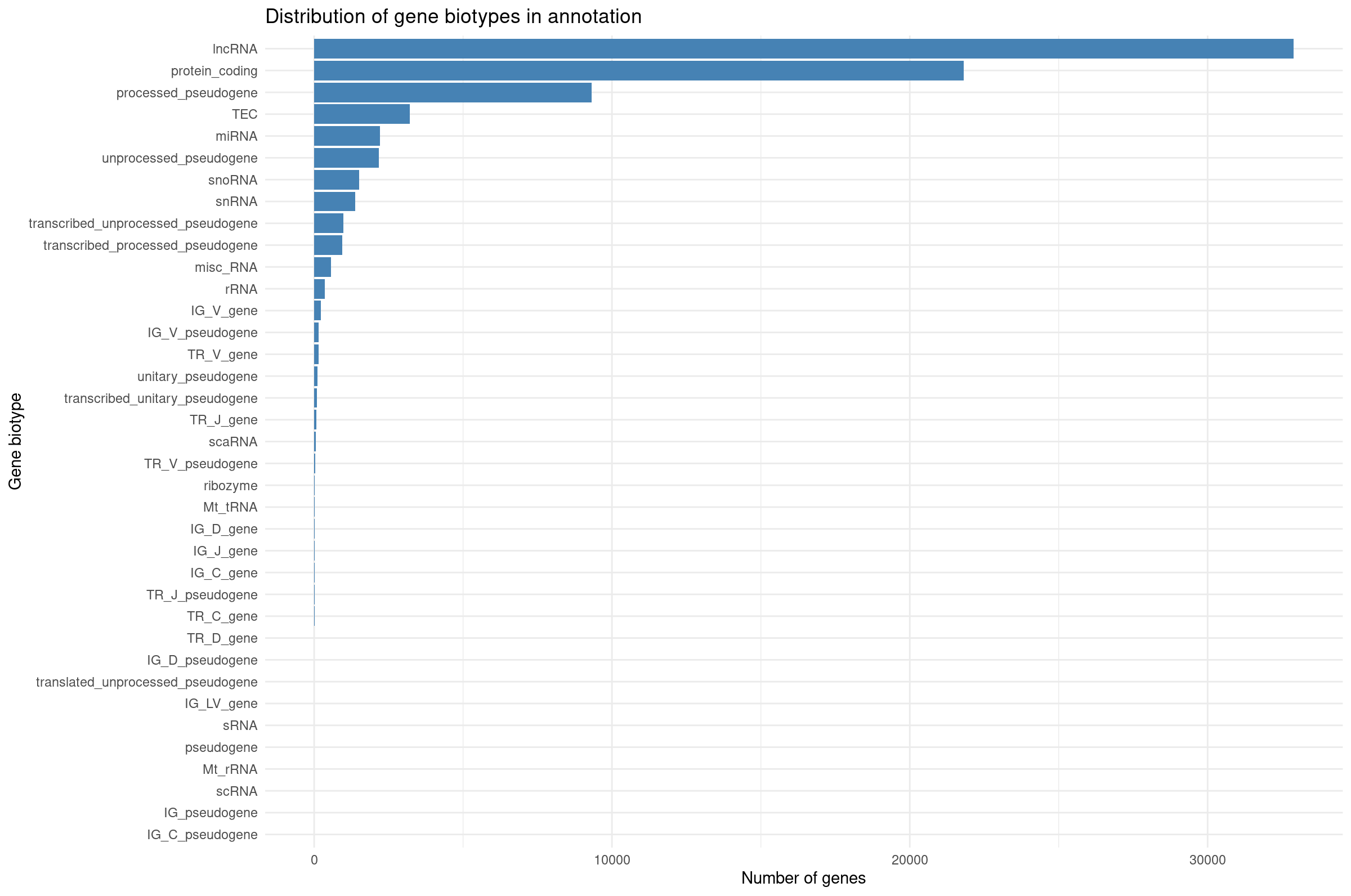
Visualizing biotype composition gives a sense of how many genes belong to each functional class. RNA-seq quantifies all transcribed loci, but many biotypes (snRNA, TEC, pseudogenes) are not suitable for differential expression with DESeq2 because they tend to be lowly expressed or unstable. This motivates filtering to protein-coding genes for QC and visualization.
Filter to protein coding genes and apply group-aware expression filtering:
R
# Filter to protein-coding genes
cts_pc <- cts_annot %>%
    filter(gene_biotype == "protein_coding") %>%
    dplyr::select(ensembl_gene_id_version, all_of(rownames(coldata)))

# Group-aware filtering: keep genes with >= 10 counts in at least 4 samples
# (the size of the smallest experimental group)
min_samples <- 4
min_counts <- 10

cts_coding <- cts_pc %>%
    filter(rowSums(across(all_of(rownames(coldata)), ~ . >= min_counts)) >= min_samples) %>%
    column_to_rownames("ensembl_gene_id_version")

dim(cts_coding)
[1] 11330 8Why use group-aware filtering?
A simple sum filter (e.g., rowSums > 5) can be
problematic:
- A gene with 10 total counts across 8 samples averages ~1.25 counts/sample—often too noisy.
- It may inadvertently remove genes expressed in only one condition.
Group-aware filtering ensures:
- Each kept gene has meaningful expression in at least one experimental group.
- Genes with condition-specific expression are retained.
- The threshold is interpretable (“at least 10 counts in at least 4 samples”).
For exploratory analysis, we also restrict to protein-coding genes to focus on the most interpretable features.
Library size differences
We summarize total counts per sample for protein coding genes.
R
libSize <- colSums(cts_coding) %>%
  as.data.frame() %>%
  rownames_to_column("sample") %>%
  rename(total_counts = 2) %>%
  mutate(total_millions = total_counts / 1e6)

ggplot(libSize, aes(x = sample, y = total_counts)) +
  geom_col(fill = "steelblue") +
  theme_minimal() +
  labs(
    x = "Sample",
    y = "Total assigned reads",
    title = "Total reads per sample"
  ) +
  theme(
    axis.text.x = element_text(angle = 45, hjust = 1)
  )
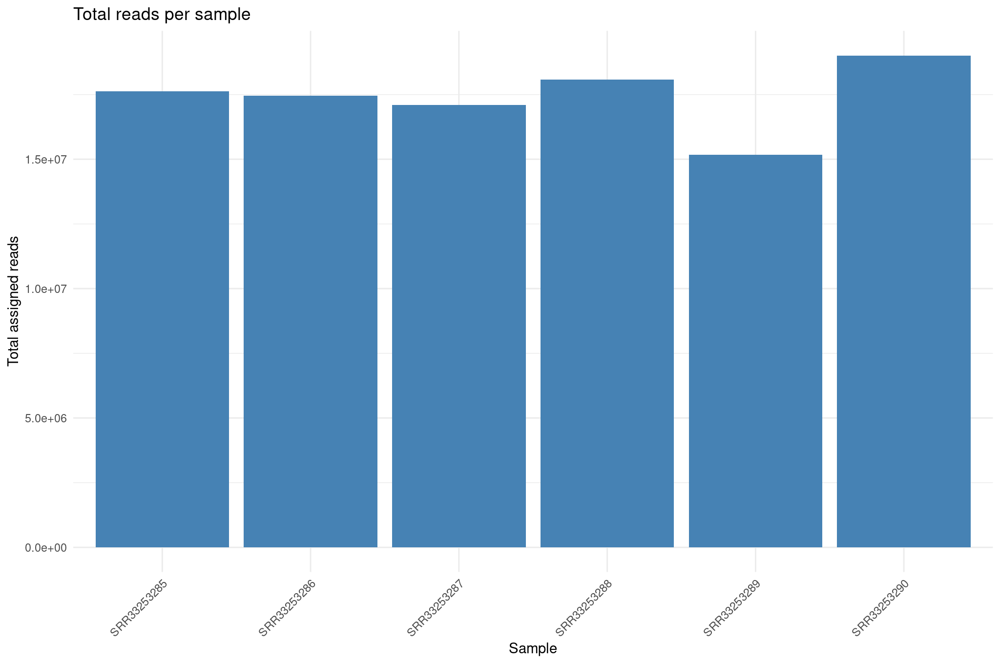
Library size differences affect normalization. Although DESeq2 corrects for this through size factors, inspecting raw library sizes ensures no sample has abnormally low sequencing depth, which could compromise downstream analyses.
Create DESeq2 object for exploratory plots
R
dds <- DESeqDataSetFromMatrix(
  countData = cts_coding,
  colData   = coldata,
  design    = ~ condition
)

dds <- estimateSizeFactors(dds)
Inspect size factors vs library size:
R
ggplot(
  data.frame(
    libSize    = colSums(assay(dds)),
    sizeFactor = sizeFactors(dds),
    Group      = dds$condition
  ),
  aes(x = libSize, y = sizeFactor, col = Group)
) +
  geom_point(size = 5) +
  theme_bw() +
  labs(x = "Library size", y = "Size factor")
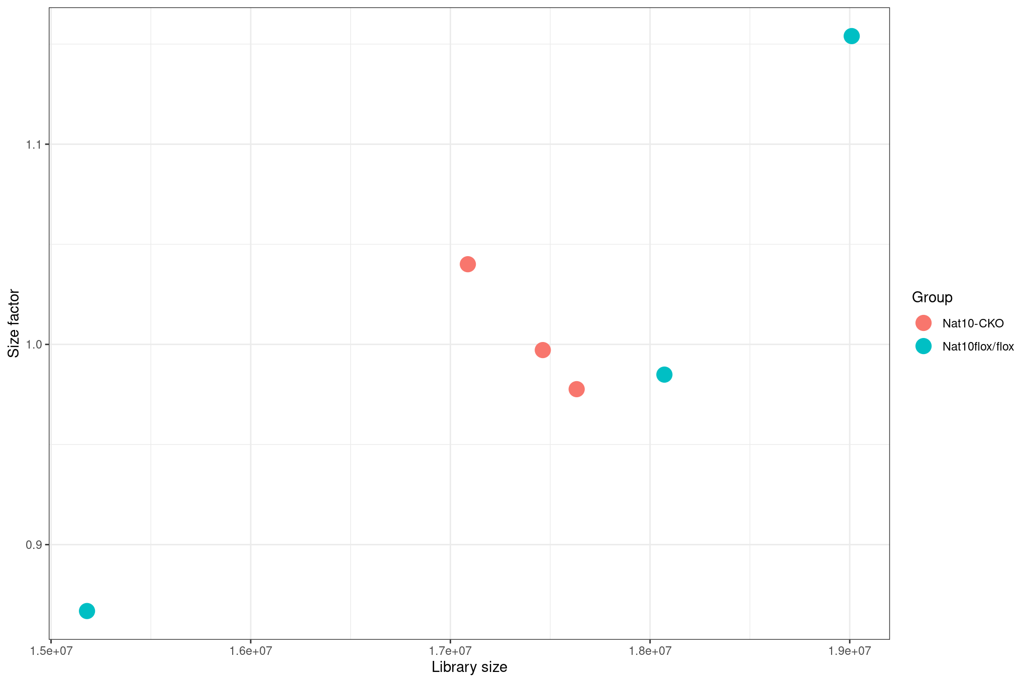
Variance stabilization and mean SD plots
Raw count data have a strong mean–variance dependency: low count genes have high variance, and high count genes show lower relative variability. This makes Euclidean distance and PCA misleading on raw counts. VST removes this dependency so that downstream clustering is biologically meaningful rather than driven by count scale.
Inspect mean vs standard deviation plot before transformation:
R
meanSdPlot(assay(dds), ranks = FALSE)
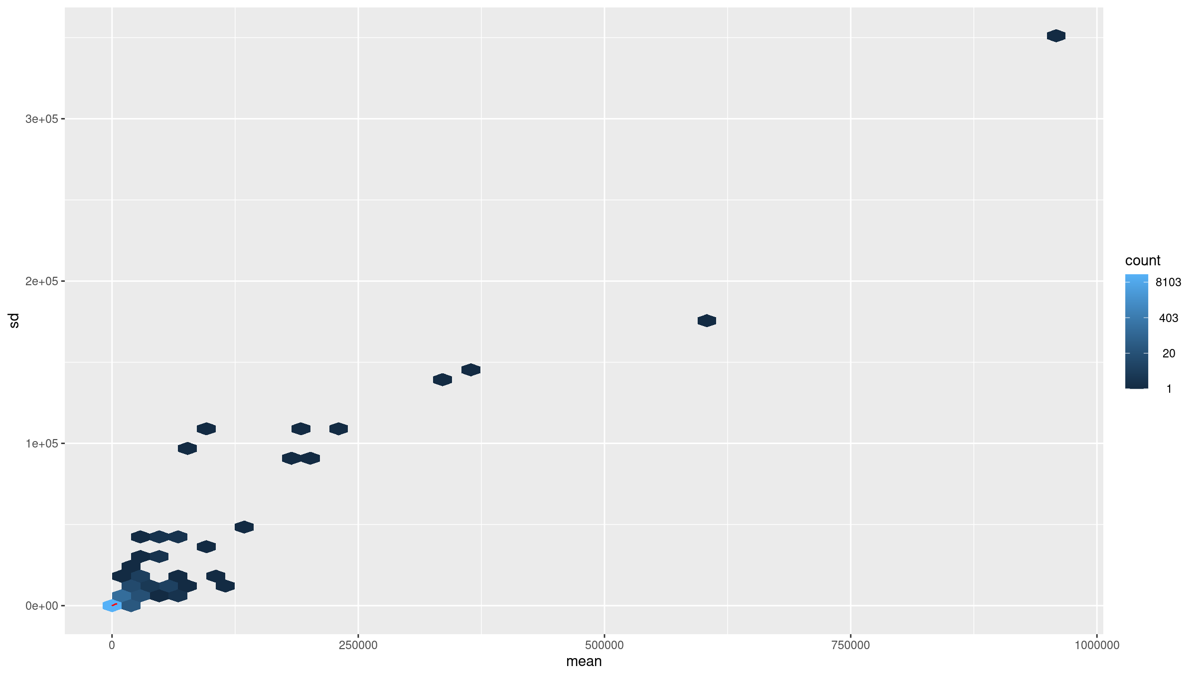
Apply variance stabilizing transform (VST):
R
vsd <- DESeq2::vst(dds, blind = TRUE)
meanSdPlot(assay(vsd), ranks = FALSE)
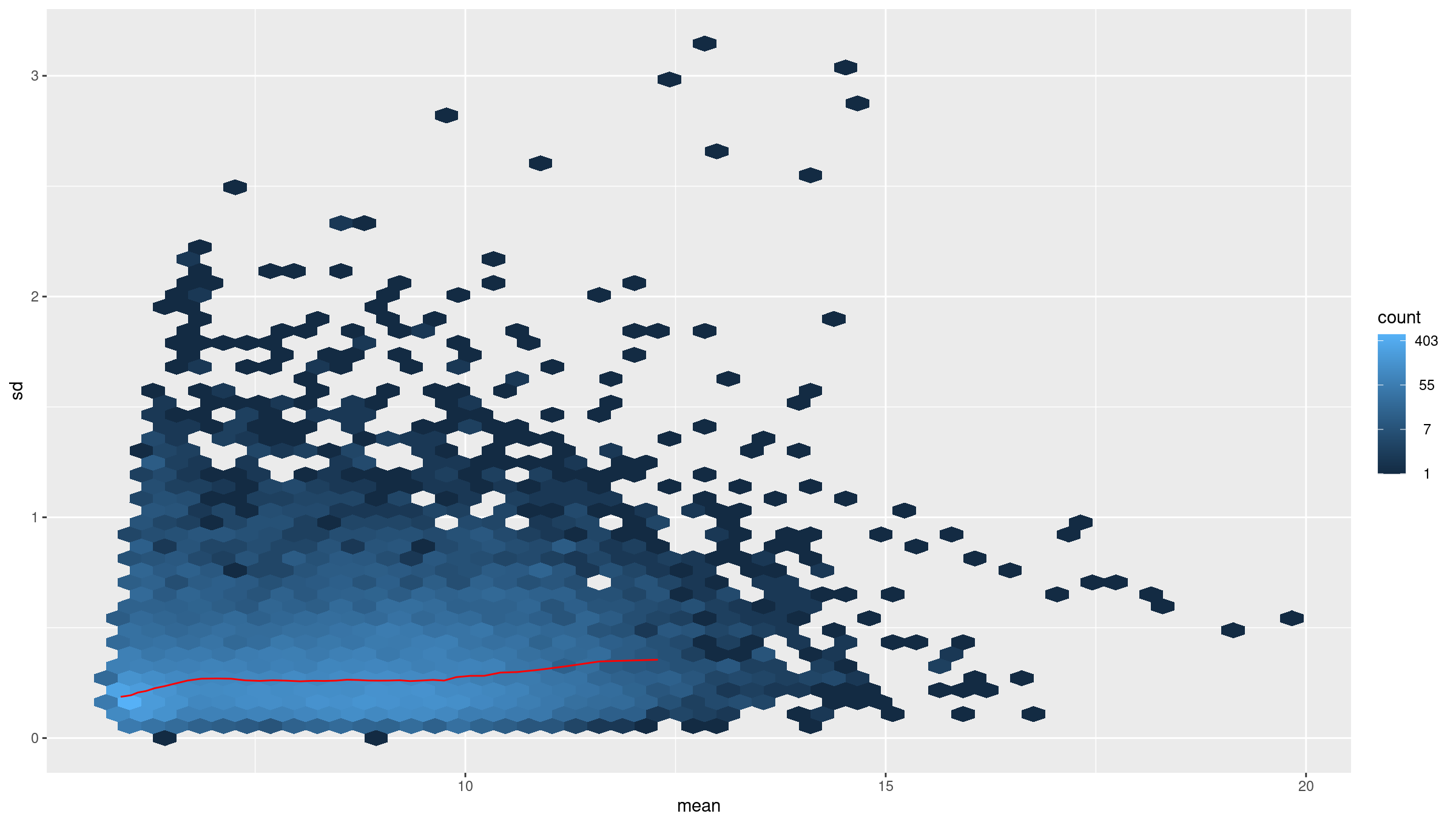
Why use VST
Counts have mean dependent variance. Variance stabilizing transform (VST) makes the variance roughly constant across the range, which improves distance based methods and PCA.
Sample to sample distances
The distance heatmap helps answer a key question: Do samples group by biological condition or by an unwanted variable (batch, sequencing run, contamination)? This is one of the fastest ways to detect outliers.
R
sampleDists       <- dist(t(assay(vsd)))
sampleDistMatrix  <- as.matrix(sampleDists)
rownames(sampleDistMatrix) <- colnames(vsd)
colnames(sampleDistMatrix) <- NULL
colors <- colorRampPalette(rev(brewer.pal(9, "Blues")))(255)

pheatmap(
  sampleDistMatrix,
  clustering_distance_rows = sampleDists,
  clustering_distance_cols = sampleDists,
  col                      = colors
)
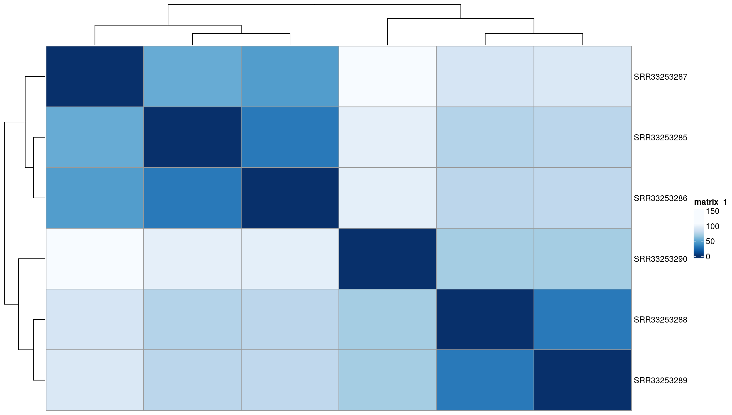
PCA on top variable genes
PCA projects samples into low-dimensional space and reveals dominant sources of variation. Ideally, samples separate by biological condition along one of the top PCs. If not, the signal from the condition may be weak or confounded by other factors.
R
rv <- rowVars(assay(vsd))
select <- order(rv, decreasing = TRUE)[seq_len(min(500, length(rv)))]

pca <- prcomp(t(assay(vsd)[select, ]))
percentVar <- pca$sdev ^ 2 / sum(pca$sdev ^ 2)

intgroup    <- "condition"
intgroup.df <- as.data.frame(colData(vsd)[, intgroup, drop = FALSE])

group <- if (length(intgroup) == 1) {
  factor(apply(intgroup.df, 1, paste, collapse = " : "))
}

d <- data.frame(
  PC1 = pca$x[, 1],
  PC2 = pca$x[, 2],
  intgroup.df,
  name = colnames(vsd)
)

ggplot(d, aes(PC1, PC2, color = condition)) +
  scale_shape_manual(values = 1:12) +
  scale_color_manual(values = c(
    "WT_mock" = "#00b462",
    "WT_IR"   = "#980c80"
  )) +
  theme_bw() +
  theme(legend.title = element_blank()) +
  geom_point(size = 2, stroke = 2) +
  geom_text_repel(aes(label = name)) +
  xlab(paste("PC1", round(percentVar[1] * 100, 2), "% variance")) +
  ylab(paste("PC2", round(percentVar[2] * 100, 2), "% variance"))
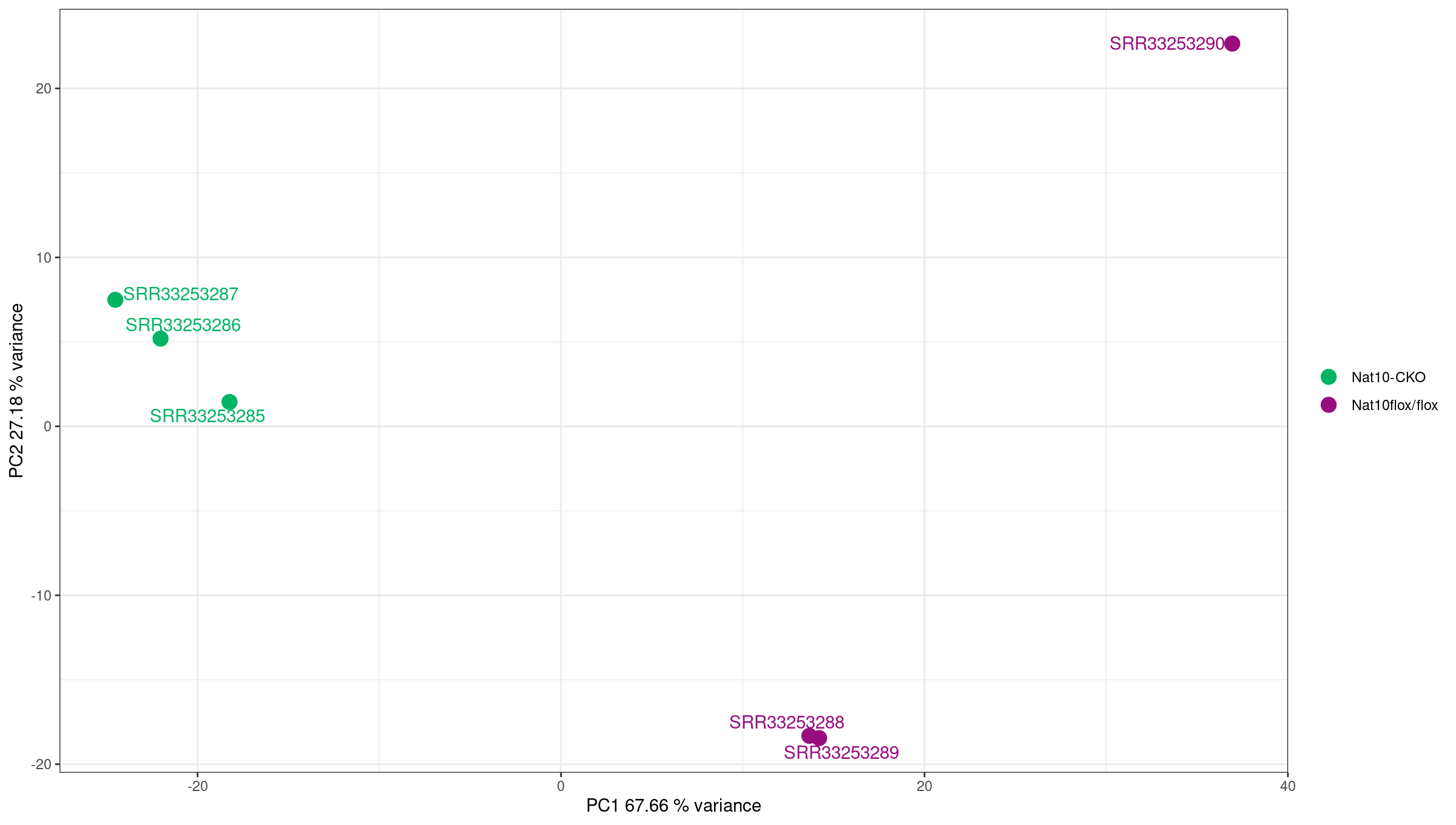
Using PCA to detect batch effects
PCA is one of the most powerful tools for detecting batch effects—unwanted technical variation from sample processing, sequencing runs, or other non-biological factors.
What to look for:
- Good: Samples separate primarily by biological condition (treatment, genotype).
- Concerning: Samples cluster by processing date, sequencing lane, or technician instead of biology.
- Red flag: PC1 captures technical variation rather than the condition of interest.
If you detect batch effects:
-
Include batch in the design formula if batch is known:
R
design = ~ batch + condition Use batch correction tools like
ComBat-seqorsvafor complex batch structures.Never simply remove batch-affected samples without understanding the underlying cause.
In this dataset, samples cluster cleanly by condition, indicating no obvious batch effects.
Exercise: interpret exploratory plots
Using the library size, distance heatmap, and PCA:
- Are there any obvious outlier samples?
- Do replicates from the same condition cluster together?
- Does any sample look inconsistent with its metadata label?
- Is there evidence of batch effects (samples clustering by non-biological factors)?
Example interpretation:
- Library sizes are comparable across samples and fall within a narrow range.
- Samples cluster by condition (mock vs IR-treated) in both distance heatmaps and PCA.
- No sample appears as a clear outlier relative to its group.
- No batch effects are apparent—PC1 separates by experimental condition, not technical factors.
Differential gene expression analysis
For DE testing we use the full count matrix
(cts) without filtering by biotype. This preserves all
features counted by featureCounts.
R
dds <- DESeqDataSetFromMatrix(
  countData = cts_coding,
  colData   = coldata,
  design    = ~ condition
)
You can either run the individual DESeq2 steps:
R
dds <- estimateSizeFactors(dds)
dds <- estimateDispersions(dds)
dds <- nbinomWaldTest(dds)
Above three steps can be run together using the DESeq
function:
R
dds <- DESeq(dds)
estimating size factors
  Note: levels of factors in the design contain characters other than
  letters, numbers, '_' and '.'. It is recommended (but not required) to use
  only letters, numbers, and delimiters '_' or '.', as these are safe characters
  for column names in R. [This is a message, not a warning or an error]
estimating dispersions
gene-wise dispersion estimates
mean-dispersion relationship
  Note: levels of factors in the design contain characters other than
  letters, numbers, '_' and '.'. It is recommended (but not required) to use
  only letters, numbers, and delimiters '_' or '.', as these are safe characters
  for column names in R. [This is a message, not a warning or an error]
final dispersion estimates
fitting model and testing
Inspect dispersion estimates:
R
plotDispEsts(dds)
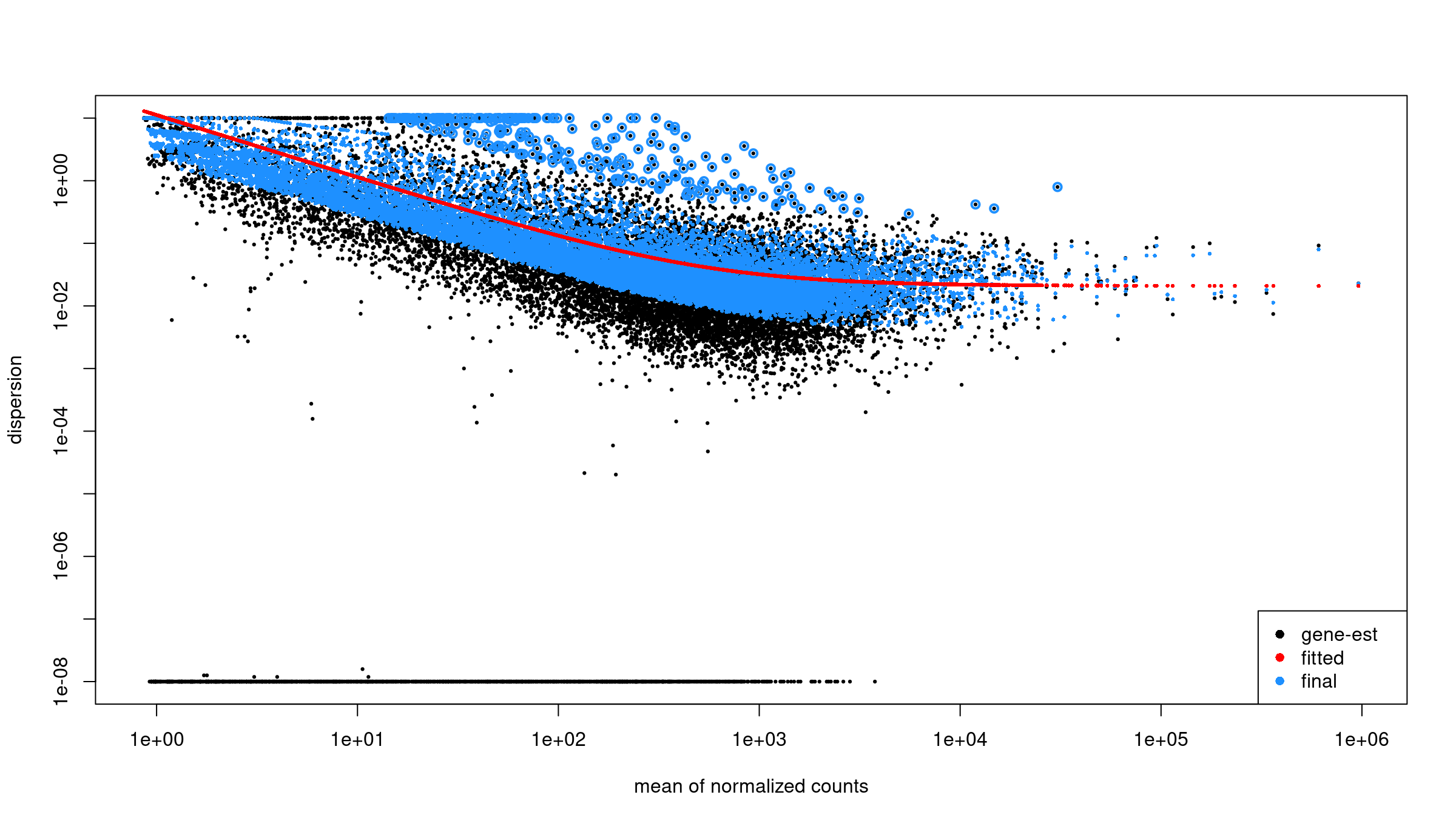
Obtain results for the contrast of interest (WT_IR vs
WT_mock):
R
res <-
  results(
    dds,
    contrast = c(
      "condition",
      "WT_IR",
      "WT_mock"
    )
  )

summary(res)
TXT
out of 11330 with nonzero total read count
adjusted p-value < 0.1
LFC > 0 (up)       : 3317, 29%
LFC < 0 (down)     : 3260, 29%
outliers [1]       : 0, 0%
low counts [2]     : 0, 0%
(mean count < 7)
[1] see 'cooksCutoff' argument of ?results
[2] see 'independentFiltering' argument of ?results
Order the results by p value to see the top DE genes:
R
head(res[order(res$pvalue), ])
log2 fold change (MLE): condition WT_IR vs WT_mock
Wald test p-value: condition WT_IR vs WT_mock
DataFrame with 6 rows and 6 columns
                       baseMean log2FoldChange     lfcSE      stat       pvalue         padj
                      <numeric>      <numeric> <numeric> <numeric>    <numeric>    <numeric>
ENSMUSG00000026581.15  2412.406       -2.80863 0.0812517  -34.5671 7.89898e-262 8.94955e-258
ENSMUSG00000021668.16   869.712        3.75461 0.1109288   33.8470 4.01308e-251 2.27341e-247
ENSMUSG00000075122.6    614.418        4.47065 0.1336974   33.4386 3.77523e-245 1.42578e-241
ENSMUSG00000004085.15   833.506        4.21081 0.1293034   32.5654 1.26916e-232 3.59488e-229
ENSMUSG00000020184.16  1619.577        2.82923 0.0906311   31.2170 6.26193e-214 1.41895e-210
ENSMUSG00000072825.13   724.296        4.73072 0.1518464   31.1546 4.39181e-213 8.29321e-210
Each row represents one gene. Key columns: baseMean:
average normalized count across all samples log2FoldChange:
direction and magnitude of change between groups pvalue /
padj: statistical significance after multiple testing
correction Genes with NA values often have too few reads to
estimate dispersion and should not be interpreted.
Apply log fold change shrinkage
The raw log2 fold change estimates from DESeq2 can be noisy for genes with low counts. Shrinkage improves these estimates.
First, check the available coefficient names:
R
resultsNames(dds)
[1] "Intercept" "condition_WT_mock_vs_WT_IR"Apply shrinkage using apeglm (recommended for standard
two-group comparisons):
R
res_shrunk <- lfcShrink(
    dds,
    coef = "condition_WT_mock_vs_WT_IR",
    type = "apeglm"
)

summary(res_shrunk)
out of 11330 with nonzero total read count
adjusted p-value < 0.1
LFC > 0 (up)       : 3260, 29%
LFC < 0 (down)     : 3317, 29%
outliers [1]       : 0, 0%
low counts [2]     : 0, 0%
(mean count < 7)
[1] see 'cooksCutoff' argument of ?results
[2] see 'independentFiltering' argument of ?resultsWhy shrink log fold changes?
Genes with low counts can have unreliably large fold changes. Shrinkage:
- Reduces noise in LFC estimates for lowly-expressed genes.
- Improves gene ranking for downstream analyses (e.g., GSEA).
- Does not affect p-values or significance calls.
Choosing a shrinkage method:
-
apeglm(recommended): Fast, well-calibrated, uses coefficient name (coef). -
ashr: Required for complex contrasts that can’t be specified withcoef. -
normal: Legacy method, generally not recommended.
For downstream analyses, we’ll use the shrunken results:
R
res <- res_shrunk
Create a summary table:
R
log2fc_cut <- log2(1.5)

res_df <- as.data.frame(res)

summary_table <- tibble(
    total_genes = nrow(res_df),
    sig = sum(res_df$padj < 0.05, na.rm = TRUE),
    up  = sum(res_df$padj < 0.05 & res_df$log2FoldChange >  log2fc_cut, na.rm = TRUE),
    down= sum(res_df$padj < 0.05 & res_df$log2FoldChange < -log2fc_cut, na.rm = TRUE)
)
print(summary_table)
Output:
# A tibble: 1 × 4
  total_genes   sig    up  down
        <int> <int> <int> <int>
1       11330  5967  1802  1795
Keep gene IDs:
R
res_df <- as.data.frame(res)
res_df$ensembl_gene_id_version <- rownames(res_df)
Joining results with expression and annotation
Get normalized counts:
R
norm_counts    <- counts(dds, normalized = TRUE)
norm_counts_df <- as.data.frame(norm_counts)
norm_counts_df$ensembl_gene_id_version <- rownames(norm_counts_df)
Join DE results, normalized counts, and annotation:
R
res_annot <- res_df %>%
  dplyr::left_join(norm_counts_df,
                   by = "ensembl_gene_id_version") %>%
  dplyr::left_join(mart,
                   by = "ensembl_gene_id_version")
Joining normalized counts and annotation makes the output
biologically interpretable. The final table becomes a comprehensive
results object containing: - gene identifiers -
gene symbols - functional descriptions -
differential expression statistics -
normalized expression values This is the format most
researchers expect when examining results or importing them into
downstream tools.
Define significance labels for plotting:
R
log2fc_cut <- log2(1.5)

res_annot <- res_annot %>%
  dplyr::mutate(
    label = dplyr::coalesce(external_gene_name, ensembl_gene_id_version),
    sig = dplyr::case_when(
      padj <= 0.05 & log2FoldChange >=  log2fc_cut ~ "up",
      padj <= 0.05 & log2FoldChange <= -log2fc_cut ~ "down",
      TRUE ~ "ns"
    )
  )
Visualization: volcano plot
The volcano plot summarizes statistical significance
(padj) and effect size (log2FoldChange)
simultaneously. Genes far left or right show strong expression
differences. Genes high on the plot pass stringent significance
thresholds. Labels help identify the most biologically meaningful
genes.
R
ggplot(
  res_annot,
  aes(
    x     = log2FoldChange,
    y     = -log10(padj),
    col   = sig,
    label = label
  )
) +
  geom_point(alpha = 0.6) +
  scale_color_manual(values = c(
    "up"   = "firebrick",
    "down" = "dodgerblue3",
    "ns"   = "grey70"
  )) +
  geom_text_repel(
    data = dplyr::filter(res_annot, sig != "ns"),
    max.overlaps       = 12,
    min.segment.length = Inf,
    box.padding        = 0.3,
    seed               = 42,
    show.legend        = FALSE
  ) +
  theme_classic() +
  xlab("log2 fold change") +
  ylab("-log10 adjusted p value") +
  ggtitle("Volcano plot: WT_IR vs WT_mock")
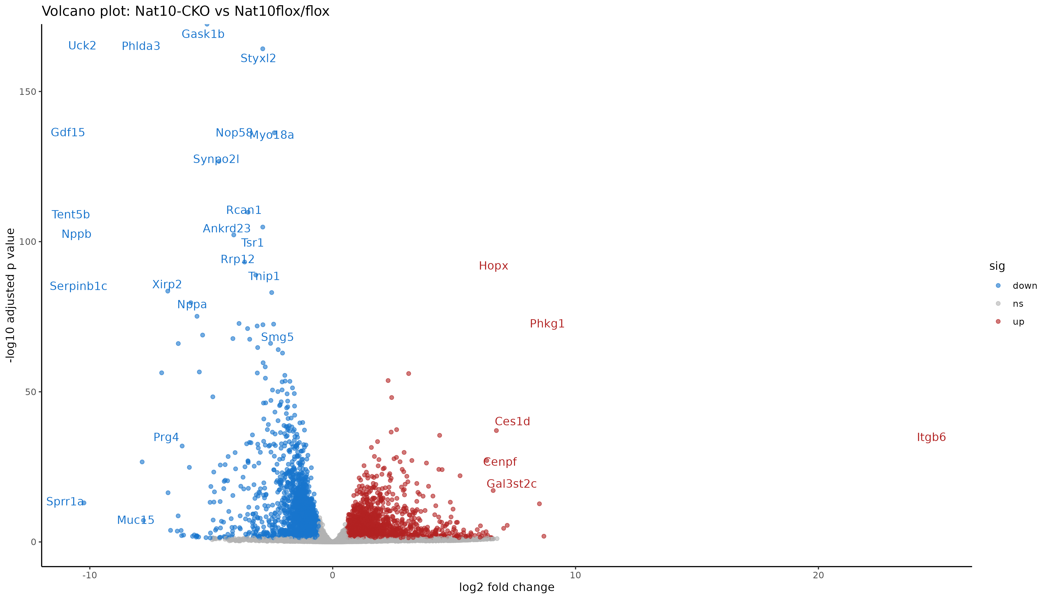
Interpreting the volcano
Points to the right are higher in IR-treated samples (upregulated by radiation), to the left are higher in mock (downregulated by radiation). Points near the top have stronger statistical support (small adjusted p values). Colored points mark genes that pass both fold change and padj thresholds.
Saving results
Saving both the full table and the significant subset allows flexibility: - The full table is needed for pathway analyses and reproducibility. - The subset table focuses on interpretable and biologically meaningful DE genes.
R
readr::write_tsv(
  res_annot,
  "results/deseq2/DESeq2_results_joined.tsv"
)
Filter to significant genes (padj ≤ 0.05 and fold change ≥ 1.5):
R
sig_res <- res_annot %>%
  dplyr::filter(
    padj <= 0.05,
    abs(log2FoldChange) >= log2fc_cut
  )

readr::write_tsv(
  sig_res,
  "results/deseq2/DESeq2_results_sig.tsv"
)
Save the DESeq2 object for downstream analysis:
R
saveRDS(dds, "results/deseq2_results/dds_featurecounts.rds")
Exercise: explore top DE genes
Using sig_res:
- Which genes have the largest positive log2 fold change.
- Which genes have the largest negative log2 fold change.
- Are any of the top genes known p53 targets or DNA damage response genes.
Example interpretation:
- Strongly upregulated genes should include canonical p53 targets such as Cdkn1a (p21), Mdm2, Bax, and Bbc3 (Puma).
- DNA damage response genes like Gadd45a should be upregulated.
- Cross-referencing top hits with p53 target databases confirms our analysis is working correctly.
Summary
- Counts and sample metadata must be aligned before building DESeq2 objects.
- Biotype annotation allows restriction to protein coding genes for exploratory QC.
- Variance stabilizing transform, distance heatmaps, and PCA help detect outliers and batch effects.
- DESeq2 provides a complete pipeline from raw counts to differential expression.
- Joining DE results with normalized counts and gene annotation yields a useful final table.
- Volcano plots summarize differential expression using fold change and adjusted p values.
Content from B. Differential expression using DESeq2 (Kallisto pathway)
Last updated on 2026-06-16 | Edit this page
Estimated time: 85 minutes
Overview
Questions
- How do we import transcript-level quantification from Kallisto into DESeq2?
- What exploratory analyses should we perform before differential expression testing?
- How do we perform differential expression analysis with DESeq2 using tximport data?
- How do we visualize and interpret DE results from transcript-based quantification?
- What are the key differences between genome-based and transcript-based DE workflows?
Objectives
- Load tximport data from Kallisto quantification into DESeq2.
- Perform quality control visualizations (boxplots, density plots, PCA).
- Apply variance stabilizing transformation for exploratory analysis.
- Run differential expression analysis with appropriate contrasts.
- Create volcano plots to visualize DE results.
- Export annotated DE results for downstream analysis.
Attribution
This section is adapted from materials developed by Michael Gribskov, Professor of Computational Genomics & Systems Biology at Purdue University.
Original and related materials are available via the CGSB Wiki: https://cgsb.miraheze.org/wiki/Main_Page
Introduction
In Episode 04b, we quantified transcript expression using Kallisto and summarized the results to gene-level counts using tximport. In this episode, we use those gene-level estimates for differential expression analysis with DESeq2.
The workflow follows the same general pattern as Episode 05 (genome-based), but with important differences:
-
Input data: We use the
txiobject from tximport rather than raw counts from featureCounts. -
Count handling: Kallisto estimates are model-based
(not integer counts), and DESeq2 handles this appropriately via
DESeqDataSetFromTximport(). - Bootstrap support: Kallisto’s uncertainty estimates (from bootstraps) can be used with sleuth for transcript-level DE.
When to use this pathway
Use this transcript-based workflow when:
- You quantified with Salmon, Kallisto, or similar tools.
- You want to leverage transcript-level bias corrections.
- You did not generate BAM files and cannot use featureCounts.
The genome-based workflow (Episode 05) is preferred when you have BAM files and need splice junction information or plan to visualize alignments.
What you need for this episode
-
txi.rdsfile generated from tximport in Episode 04b - A
samples.csvfile describing the experimental groups - RStudio session via Open OnDemand
If you haven’t created the sample metadata file, create
scripts/samples.csv with:
sample,condition
WT_Bcell_mock_rep1,WT_mock
WT_Bcell_mock_rep2,WT_mock
WT_Bcell_mock_rep3,WT_mock
WT_Bcell_mock_rep4,WT_mock
WT_Bcell_IR_rep1,WT_IR
WT_Bcell_IR_rep2,WT_IR
WT_Bcell_IR_rep3,WT_IR
WT_Bcell_IR_rep4,WT_IR
Create a results directory:
Step 1: Load packages and data
Start your RStudio session via Open OnDemand as described in Episode 05, then load the required packages:
R
library(DESeq2)
library(tximportData)
library(ggplot2)
library(reshape2)
library(pheatmap)
library(RColorBrewer)
library(ggrepel)
library(readr)
library(dplyr)
# Construct the path dynamically
work_dir <- file.path("/scratch/negishi", Sys.getenv("USER"), "rnaseq-workshop")
setwd(work_dir)
Load the tximport object created in Episode 04b:
R
txi <- readRDS("results/kallisto_quant/txi.rds")
Examine the structure of the tximport object:
R
names(txi)
[1] "abundance" "counts" "infReps" "length" "countsFromAbundance"R
head(txi$counts)
                      WT_Bcell_IR_rep1 WT_Bcell_IR_rep2 WT_Bcell_IR_rep3 WT_Bcell_IR_rep4 WT_Bcell_mock_rep1 WT_Bcell_mock_rep2 WT_Bcell_mock_rep3
ENSMUSG00000000001.5         387.39815         329.4356     737.97311964        654.17550           687.1189          620.35065          661.35411
ENSMUSG00000000003.16          0.00000           1.0000       0.00000000          0.00000             0.0000            0.00000            0.00000
ENSMUSG00000000028.16         32.81579          20.0000      36.63144821         29.71743            53.5750           36.92104           39.00000
ENSMUSG00000000031.20          0.00000           0.0000       0.09733145          0.00000             0.0000            0.00000            0.00000
ENSMUSG00000000037.18          2.00000           3.0000       1.28018005          8.00000             1.0000            0.00000            1.58711
ENSMUSG00000000049.12          0.00000           0.0000       0.00000000          0.00000             0.0000            0.00000            0.00000
                      WT_Bcell_mock_rep4
ENSMUSG00000000001.5            704.8851
ENSMUSG00000000003.16             0.0000
ENSMUSG00000000028.16            36.0000
ENSMUSG00000000031.20             0.0000
ENSMUSG00000000037.18             0.0000
ENSMUSG00000000049.12 0.0000Understanding the tximport object
The txi object contains several components:
- counts: Gene-level estimated counts (used by DESeq2).
- abundance: Gene-level TPM values (within-sample normalized).
- length: Average transcript length per gene (used for length bias correction).
-
countsFromAbundance: Method used to generate counts
(default:
"no").
When using DESeqDataSetFromTximport(), the
length matrix is automatically used to correct for
gene-length bias during normalization. This is why we use the default
countsFromAbundance = "no" in Episode 04b—DESeq2 handles
length correction internally, so pre-scaling counts would apply the
correction twice.
Load sample metadata:
R
coldata <- read.csv(
    "scripts/samples.csv",
    row.names = 1,
    header = TRUE,
    stringsAsFactors = TRUE
)
coldata$condition <- as.factor(coldata$condition)
coldata <- coldata[colnames(txi$counts), , drop = FALSE]
coldata
                   condition
WT_Bcell_IR_rep1       WT_IR
WT_Bcell_IR_rep2       WT_IR
WT_Bcell_IR_rep3       WT_IR
WT_Bcell_IR_rep4       WT_IR
WT_Bcell_mock_rep1   WT_mock
WT_Bcell_mock_rep2   WT_mock
WT_Bcell_mock_rep3   WT_mock
WT_Bcell_mock_rep4   WT_mock
Verify that sample names match between tximport and metadata:
R
all(colnames(txi$counts) == rownames(coldata))
[1] TRUEStep 2: Create DESeq2 object from tximport
The key difference from the genome-based workflow is using
DESeqDataSetFromTximport() instead of
DESeqDataSetFromMatrix():
R
dds <- DESeqDataSetFromTximport(
    txi,
    colData = coldata,
    design = ~ condition
)
Why use DESeqDataSetFromTximport?
This function:
- Automatically handles non-integer counts from Salmon/Kallisto.
- Preserves transcript length information for accurate normalization.
- Incorporates the
txi$lengthmatrix to account for gene-length bias.
Using DESeqDataSetFromMatrix() with tximport counts
would lose this information.
Filter lowly expressed genes using group-aware filtering:
R
# Group-aware filtering: keep genes with >= 10 counts in at least 4 samples
# (the size of the smallest experimental group)
min_samples <- 4
min_counts <- 10
keep <- rowSums(counts(dds) >= min_counts) >= min_samples
dds <- dds[keep, ]
dim(dds)
[1] 18924 8Why use group-aware filtering?
A simple sum filter (rowSums(counts(dds)) >= 10) can
be problematic:
- A gene with 10 total counts across 8 samples averages ~1.25 counts/sample—too low to be informative.
- It may remove genes expressed in only one condition (biologically interesting!).
Group-aware filtering
(rowSums(counts >= threshold) >= min_group_size)
ensures:
- Each kept gene has meaningful expression in at least one experimental group.
- Genes with condition-specific expression are retained.
- The threshold is interpretable (e.g., “at least 10 counts in at least 4 samples”).
Estimate size factors:
R
dds <- estimateSizeFactors(dds)
head(normalizationFactors(dds))
                      WT_Bcell_IR_rep1 WT_Bcell_IR_rep2 WT_Bcell_IR_rep3 WT_Bcell_IR_rep4 WT_Bcell_mock_rep1 WT_Bcell_mock_rep2 WT_Bcell_mock_rep3
ENSMUSG00000000001.5         0.8578693        0.8520842         1.099577        1.0524525           1.059461          0.9946634          0.9552297
ENSMUSG00000000028.16        0.9455555        0.7479666         1.149805        0.9882356           1.071439          1.0191038          0.9154327
ENSMUSG00000000056.8         0.8580737        0.8528464         1.101744        1.0540656           1.058546          0.9930345          0.9540278
ENSMUSG00000000078.8         0.8580503        0.8527592         1.101496        1.0538811           1.058650          0.9932207          0.9541651
ENSMUSG00000000085.17        0.7941016        0.7697798         1.199288        1.0181546           1.163680          0.9580967          1.0675296
ENSMUSG00000000088.8         0.8537054        0.8364591         1.055812        1.0199231           1.078562          1.0286198          0.9803416
                      WT_Bcell_mock_rep4
ENSMUSG00000000001.5            1.174355
ENSMUSG00000000028.16           1.244899
ENSMUSG00000000056.8            1.173333
ENSMUSG00000000078.8            1.173450
ENSMUSG00000000085.17           1.125634
ENSMUSG00000000088.8            1.195682
Step 3: Exploratory data analysis
Raw count distributions
Visualize the distribution of raw counts across samples:
R
counts_melted <- melt(
    log10(counts(dds) + 1),
    varnames = c("gene", "sample"),
    value.name = "log10_count"
)

ggplot(counts_melted, aes(x = sample, y = log10_count, fill = sample)) +
    geom_boxplot(show.legend = FALSE) +
    theme_minimal() +
    labs(
        x = "Sample",
        y = "log10(count + 1)",
        title = "Raw count distributions (Kallisto)"
    ) +
    theme(axis.text.x = element_text(angle = 45, hjust = 1))
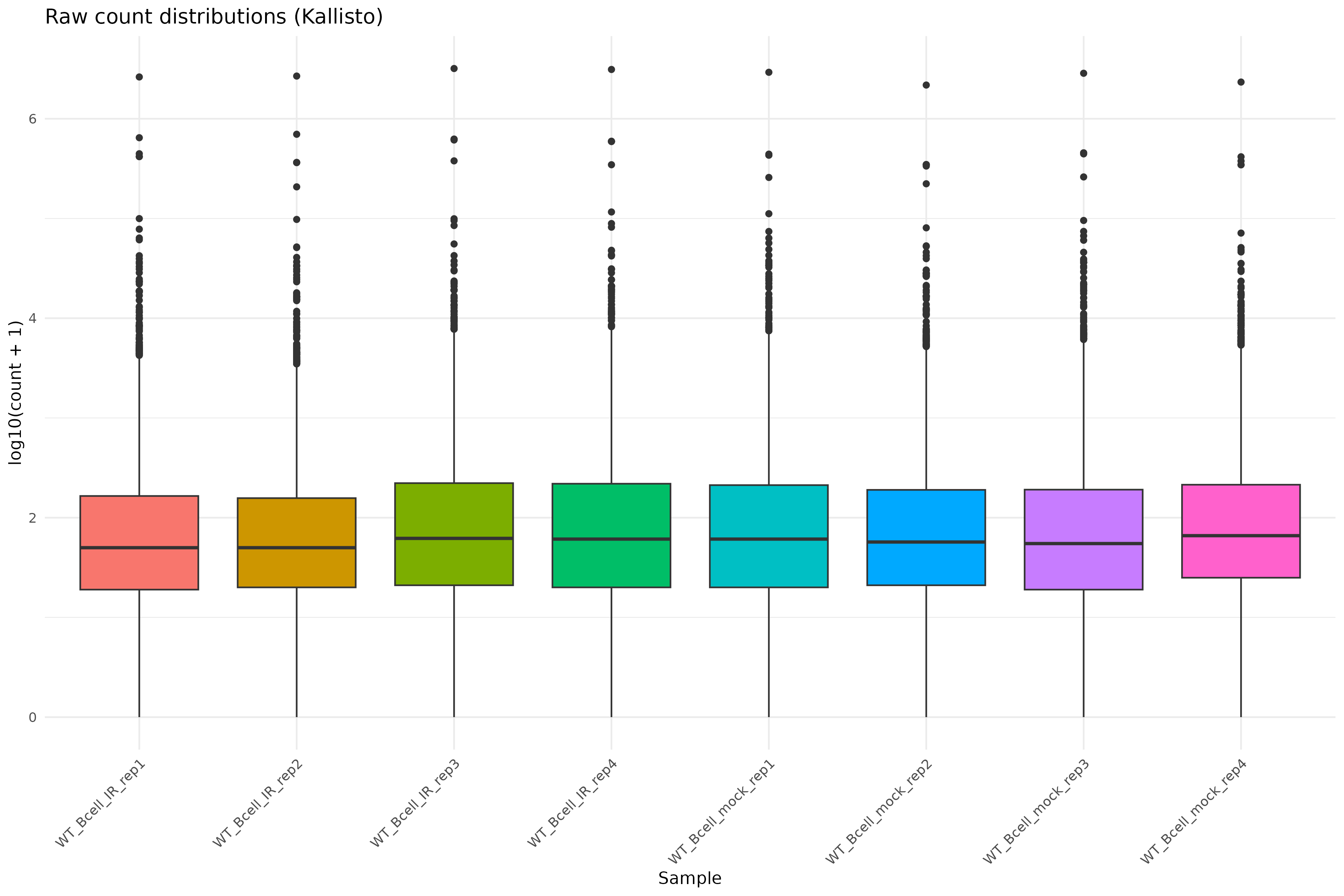
Density plot of raw counts:
R
ggplot(counts_melted, aes(x = log10_count, fill = sample)) +
    geom_density(alpha = 0.3) +
    theme_minimal() +
    labs(
        x = "log10(count + 1)",
        y = "Density",
        title = "Count density distributions"
    )
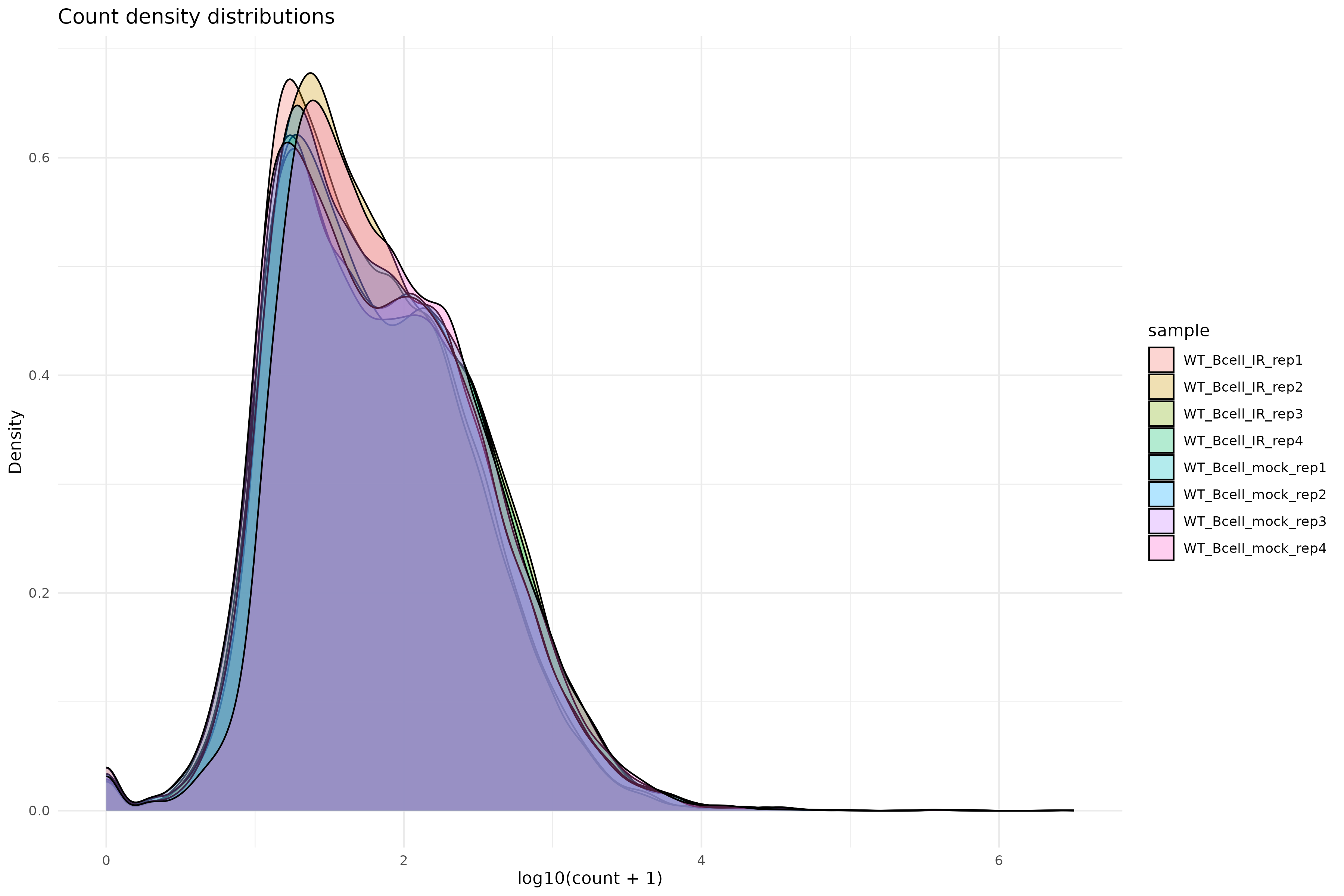
Variance stabilizing transformation
Apply VST for exploratory analysis:
R
vsd <- vst(dds, blind = TRUE)
Why use VST?
Raw counts have a strong mean-variance relationship: highly expressed genes have higher variance. VST removes this dependency, making distance-based methods (PCA, clustering) more reliable.
Setting blind = TRUE ensures the transformation is not
influenced by the experimental design, which is appropriate for quality
control.
Sample-to-sample distances
R
sampleDists <- dist(t(assay(vsd)))
sampleDistMatrix <- as.matrix(sampleDists)
rownames(sampleDistMatrix) <- colnames(vsd)
colnames(sampleDistMatrix) <- NULL
colors <- colorRampPalette(rev(brewer.pal(9, "Blues")))(255)

pheatmap(
    sampleDistMatrix,
    clustering_distance_rows = sampleDists,
    clustering_distance_cols = sampleDists,
    col = colors,
    main = "Sample distance heatmap (Kallisto)"
)
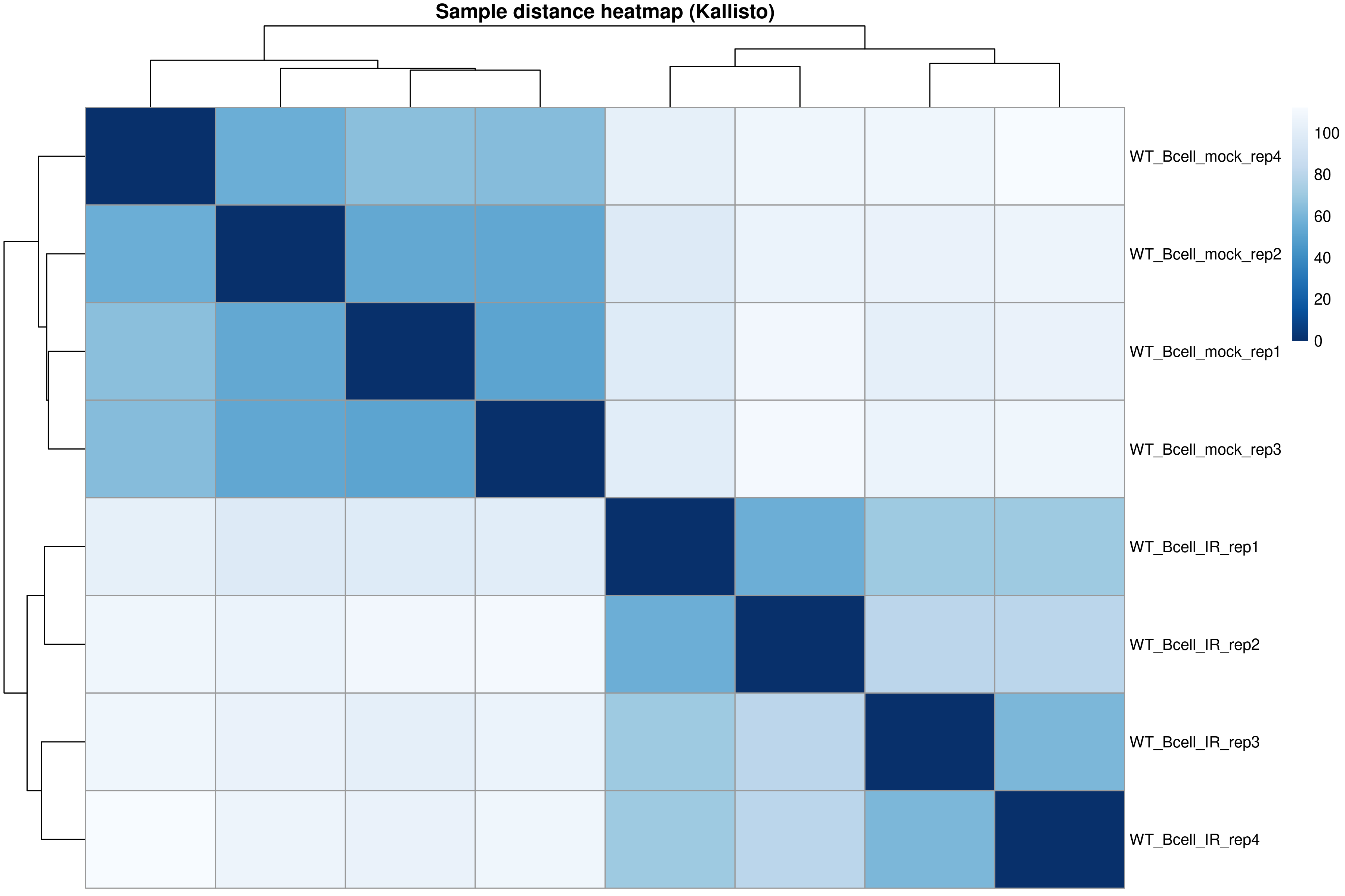
The distance heatmap shows how similar samples are to each other. Samples from the same condition should cluster together.
PCA plot
R
pcaData <- plotPCA(vsd, intgroup = "condition", returnData = TRUE)
percentVar <- round(100 * attr(pcaData, "percentVar"))

ggplot(pcaData, aes(PC1, PC2, color = condition)) +
    geom_point(size = 4) +
    geom_text_repel(aes(label = name)) +
    xlab(paste0("PC1: ", percentVar[1], "% variance")) +
    ylab(paste0("PC2: ", percentVar[2], "% variance")) +
    theme_bw() +
    ggtitle("PCA of Kallisto-quantified samples")
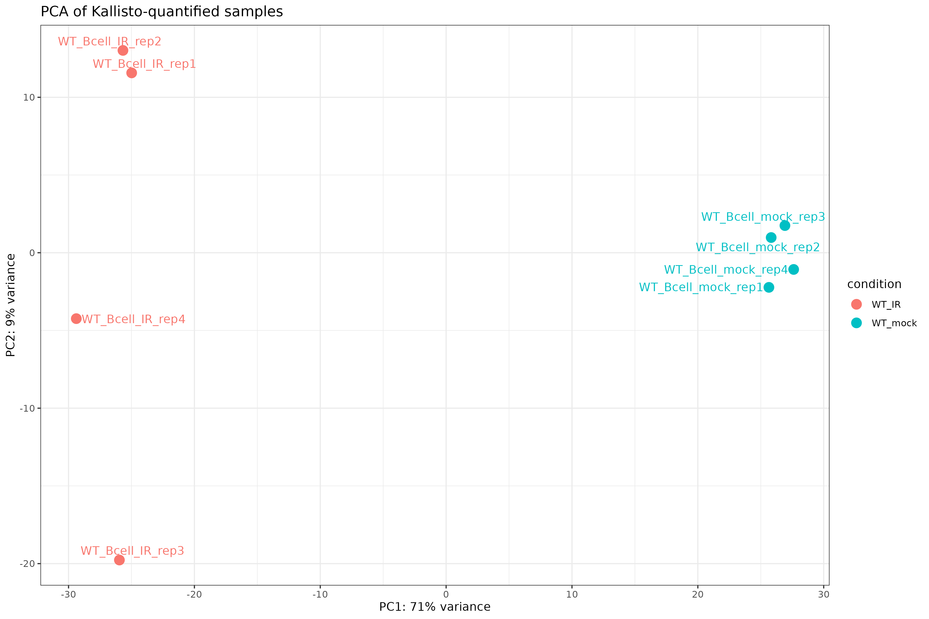
Exercise: Interpret exploratory plots
Using the distance heatmap and PCA plot:
- Do samples cluster by experimental condition?
- Are there any outlier samples that don’t group with their replicates?
- How much variance is explained by PC1? What might this represent biologically?
Example interpretation:
- Samples should cluster by condition (WT_mock vs WT_IR) in both the heatmap and PCA.
- If all replicates cluster together, there are no obvious outliers.
- PC1 typically captures the largest source of variation. If it separates conditions, the experimental treatment is the dominant signal.
Step 4: Differential expression analysis
Run the full DESeq2 pipeline:
R
dds <- DESeq(dds)
estimating size factors
estimating dispersions
gene-wise dispersion estimates
mean-dispersion relationship
final dispersion estimates
fitting model and testing
Inspect dispersion estimates:
R
plotDispEsts(dds)
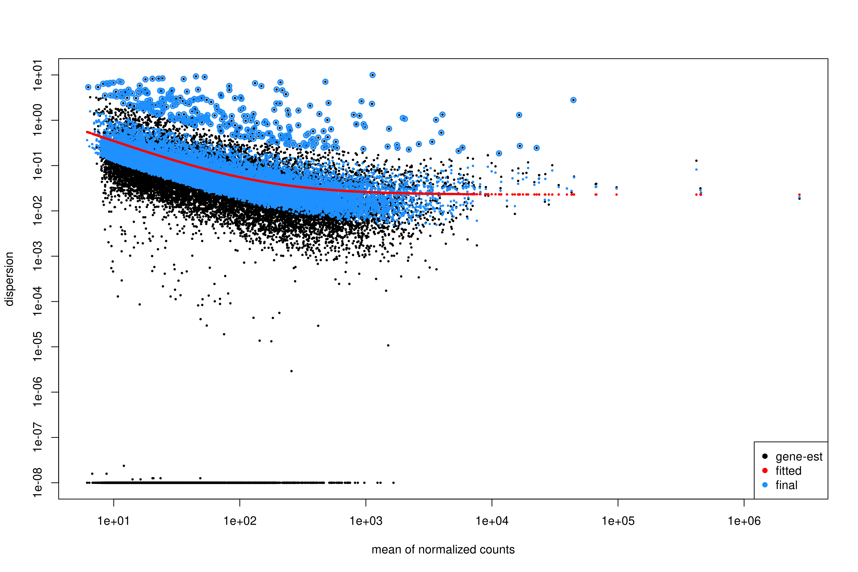
Interpreting the dispersion plot
- Black dots: Gene-wise dispersion estimates.
- Red line: Fitted trend (shrinkage target).
- Blue dots: Final shrunken estimates.
A good fit shows the red line passing through the center of the black cloud, with blue dots closer to the line than the original black dots.
Extract results for the contrast of interest:
R
res <- results(
    dds,
    contrast = c("condition", "WT_mock", "WT_IR")
)

summary(res)
out of 19693 with nonzero total read count
adjusted p-value < 0.1
LFC > 0 (up)       : 3482, 18%
LFC < 0 (down)     : 3675, 19%
outliers [1]       : 10, 0.051%
low counts [2]     : 0, 0%
(mean count < 6)
[1] see 'cooksCutoff' argument of ?results
[2] see 'independentFiltering' argument of ?results
Order results by adjusted p-value:
R
res_ordered <- res[order(res$padj), ]
head(res_ordered)
Output:
log2 fold change (MLE): condition WT_IR vs WT_mock
Wald test p-value: condition WT_IR vs WT_mock
DataFrame with 6 rows and 6 columns
                       baseMean log2FoldChange     lfcSE      stat       pvalue         padj
                      <numeric>      <numeric> <numeric> <numeric>    <numeric>    <numeric>
ENSMUSG00000004085.15   795.499        4.10779  0.157888   26.0172 3.16645e-149 6.23252e-145
ENSMUSG00000021701.9    840.251        6.34293  0.253829   24.9889 8.06388e-138 7.93607e-134
ENSMUSG00000072825.13   705.733        4.70979  0.190927   24.6680 2.35896e-134 1.54771e-130
ENSMUSG00000048458.9    820.666        5.79808  0.238203   24.3409 7.24251e-131 3.56386e-127
ENSMUSG00000028893.9    680.824        4.28171  0.179531   23.8495 1.02517e-125 4.03570e-122
ENSMUSG00000075122.6    836.194        3.74860  0.158501   23.6502 1.17375e-123 3.85048e-120
Apply log fold change shrinkage
LFC shrinkage improves estimates for genes with low counts or high dispersion.
First, check the available coefficients:
R
resultsNames(dds)
[1] "Intercept" "condition_WT_mock_vs_WT_IR"Apply shrinkage using apeglm (recommended for standard
contrasts):
R
res_shrunk <- lfcShrink(
    dds,
    coef = "condition_WT_mock_vs_WT_IR",
    type = "apeglm"
)
Why shrink log fold changes?
Genes with low counts can have unreliably large fold changes. Shrinkage:
- Reduces noise in LFC estimates.
- Improves ranking for downstream analyses (e.g., GSEA).
- Does not affect p-values or significance calls.
Choosing a shrinkage method
-
apeglm(recommended): Fast, well-calibrated, uses coefficient name (coef). -
ashr: Required for complex contrasts that can’t be specified withcoef(e.g., interaction terms). -
normal: Legacy method, generally not recommended.
For simple two-group comparisons like ours, apeglm is
preferred.
Step 5: Summarize and visualize results
Create a summary table:
R
log2fc_cut <- log2(1.5)

res_df <- as.data.frame(res_shrunk)
res_df$gene_id <- rownames(res_df)

summary_table <- tibble(
    total_genes = nrow(res_df),
    sig = sum(res_df$padj < 0.05, na.rm = TRUE),
    up = sum(res_df$padj < 0.05 & res_df$log2FoldChange > log2fc_cut, na.rm = TRUE),
    down = sum(res_df$padj < 0.05 & res_df$log2FoldChange < -log2fc_cut, na.rm = TRUE)
)

print(summary_table)
output:
# A tibble: 1 × 4
  total_genes   sig    up  down
        <int> <int> <int> <int>
1       19693  6078  2296  2448
We will attach annotations so that results are interpretable. Load gene annotation data (from Episode 02):
R
mart <-
  read.csv(
    "data/mart.tsv",
    sep = "\t",
    header = TRUE
  )

annot <-
  read.csv(
    "data/annot.tsv",
    sep = "\t",
    header = TRUE
  )
R
res_df <- as.data.frame(res)
res_df$ensembl_gene_id_version <- rownames(res_df)
Join DE results, normalized counts, and annotation:
R
res_annot <- res_df %>%
  dplyr::left_join(mart,
                   by = "ensembl_gene_id_version")
Joining normalized counts and annotation makes the output biologically interpretable. The final table becomes a comprehensive results object containing:
gene identifiersgene symbolsfunctional descriptionsdifferential expression statistics
This is the format most researchers expect when examining results or importing them into downstream tools.
Define significance labels for plotting:
R
log2fc_cut <- log2(1.5)

res_annot <- res_annot %>%
  dplyr::mutate(
    label = dplyr::coalesce(external_gene_name, ensembl_gene_id_version),
    sig = dplyr::case_when(
      padj <= 0.05 & log2FoldChange >=  log2fc_cut ~ "up",
      padj <= 0.05 & log2FoldChange <= -log2fc_cut ~ "down",
      TRUE ~ "ns"
    )
  )
Volcano plot
R
ggplot(
  res_annot,
  aes(
    x     = log2FoldChange,
    y     = -log10(padj),
    col   = sig,
    label = label
  )
) +
  geom_point(alpha = 0.6) +
  scale_color_manual(values = c(
    "up"   = "firebrick",
    "down" = "dodgerblue3",
    "ns"   = "grey70"
  )) +
  geom_text_repel(
    data = dplyr::filter(res_annot, sig != "ns"),
    max.overlaps       = 12,
    min.segment.length = Inf,
    box.padding        = 0.3,
    seed               = 42,
    show.legend        = FALSE
  ) +
  geom_hline(yintercept = -log10(0.05), linetype = "dashed", color = "grey40") +
  geom_vline(xintercept = c(-log2fc_cut, log2fc_cut), linetype = "dashed", color = "grey40") +
  theme_classic() +
  xlab("log2 fold change") +
  ylab("-log10 adjusted p value") +
  ggtitle("Volcano plot: WT_IR vs WT_mock")
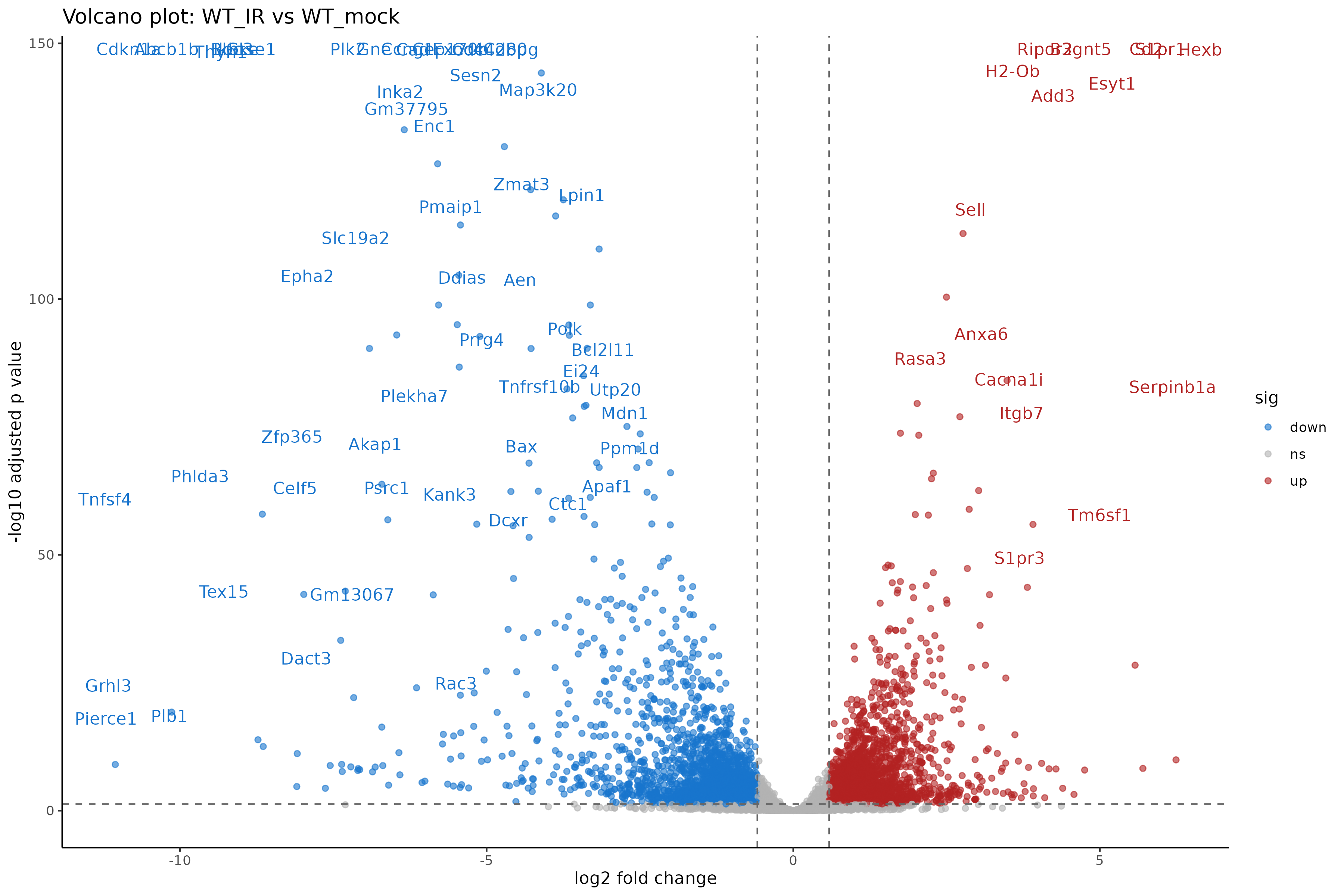
Interpreting the volcano plot
- X-axis: Direction and magnitude of change (positive = higher in WT_IR, i.e., upregulated by radiation).
- Y-axis: Statistical significance (-log10 scale, higher = more significant).
- Colored points: Genes passing both fold change and significance thresholds.
Exercise: Compare with genome-based results
If you also ran Episode 05 (genome-based workflow):
- Are the number of DE genes similar between the two approaches?
- Do the top DE genes overlap?
- Are there systematic differences in fold change estimates?
Expected observations:
- The number of DE genes should be broadly similar, though not identical.
- Most top DE genes should overlap between methods.
- Kallisto may produce slightly different LFC estimates due to its different quantification algorithm.
Both approaches are valid; consistency between them increases confidence in the results.
Step 6: Save results
Save the full results table:
R
write_tsv(
    res_df,
    "results/deseq2_kallisto/DESeq2_kallisto_results.tsv"
)
Save significant genes only:
R
sig_res <- res_df %>%
    filter(
        padj <= 0.05,
        abs(log2FoldChange) >= log2fc_cut
    )

write_tsv(
    sig_res,
    "results/deseq2_kallisto/DESeq2_kallisto_sig.tsv"
)
Save the DESeq2 object for downstream analysis:
R
saveRDS(dds, "results/deseq2_kallisto/dds_kallisto.rds")
Genome-based vs. transcript-based: Which to choose?
| Aspect | Genome-based (Ep 05) | Transcript-based (Ep 05b) |
|---|---|---|
| Input | BAM files | FASTQ files |
| Speed | Slower (alignment + counting) | Faster (pseudo-alignment) |
| Storage | Large (BAM files) | Small (abundance.tsv files) |
| Bias correction | Limited | Sequence + GC bias |
| Novel transcripts | Can detect | Cannot detect |
| Visualization | IGV compatible | No BAM files |
For standard differential expression, both methods produce comparable results. Choose based on your specific needs and available resources.
Summary
- Kallisto output is imported via
tximportand loaded withDESeqDataSetFromTximport(). - The tximport object preserves transcript length information for accurate normalization.
- Exploratory analysis (PCA, distance heatmaps) should precede differential expression testing.
- DESeq2 handles the statistical analysis identically to the genome-based workflow.
- LFC shrinkage improves fold change estimates for low-count genes.
- Results from transcript-based and genome-based workflows should be broadly concordant.
Content from Gene set enrichment analysis
Last updated on 2026-06-16 | Edit this page
Estimated time: 95 minutes
Overview
Questions
- What is over-representation analysis and how does it work statistically?
- How do we identify functional pathways and biological themes from DE genes?
- How do we run enrichment analysis for GO, KEGG, and MSigDB gene sets?
- How do we interpret and compare enrichment results across different databases?
- What are the limitations and best practices for enrichment analysis?
Objectives
- Understand the statistical basis of over-representation analysis (ORA).
- Prepare gene lists and background universes from DESeq2 results.
- Run GO enrichment using clusterProfiler and interpret ontology categories.
- Run KEGG pathway enrichment with organism-specific data.
- Perform MSigDB Hallmark enrichment for curated biological signatures.
- Produce and interpret barplots, dotplots, and enrichment maps.
- Compare results across multiple gene set databases.
Introduction
Differential expression analysis identifies individual genes that change between conditions, but interpreting long gene lists is challenging. Gene set enrichment analysis provides biological context by asking: Are genes with specific functions over-represented among the differentially expressed genes?
This episode covers over-representation analysis (ORA), the most common approach for interpreting DE results.
What you need for this episode
- DE results from Episode 05 or 05b
(
DESeq2_results_joined.tsvorDESeq2_kallisto_results.tsv) - RStudio session via Open OnDemand
- Internet connection (for KEGG queries)
Background: Understanding over-representation analysis
What is ORA?
ORA tests whether a predefined gene set contains more DE genes than expected by chance. It answers the question: If I randomly selected the same number of genes from my background, how often would I see this many genes from pathway X?
The statistical test
ORA uses the hypergeometric test (equivalent to Fisher’s exact test), which calculates the probability of observing k or more genes from a pathway given:
- N: Total genes in the background (universe)
- K: Genes in the pathway of interest
- n: Total DE genes in your list
- k: DE genes that are in the pathway
                    Pathway genes    Non-pathway genes
DE genes                 k              n - k
Non-DE genes K - k N - K - n + kThe hypergeometric distribution
The p-value represents the probability of drawing k or more pathway genes when randomly selecting n genes from a population of N genes containing K pathway members:
\[P(X \geq k) = \sum_{i=k}^{\min(K,n)} \frac{\binom{K}{i}\binom{N-K}{n-i}}{\binom{N}{n}}\]
This is a one-tailed test asking if the pathway is over-represented (enriched) in your gene list.
Multiple testing correction
With thousands of gene sets tested, many false positives would occur by chance. We apply false discovery rate (FDR) correction using the Benjamini-Hochberg method:
- Rank all p-values from smallest to largest.
- Calculate adjusted p-value: \(p_{adj} = p \times \frac{n}{rank}\)
- Filter results by adjusted p-value threshold (typically 0.05).
Why the universe matters
The background universe should include all genes that could have been detected as DE in your experiment, typically all genes tested by DESeq2.
Common mistakes: - Using the whole genome (inflates significance). - Using only expressed genes (may miss relevant pathways). - Using a different species’ gene list.
The universe defines what “expected by chance” means. An inappropriate universe leads to misleading results.
Gene set databases
Different databases capture different aspects of biology:
| Database | Description | Best for |
|---|---|---|
| GO BP | Biological Process ontology | Functional processes |
| GO MF | Molecular Function ontology | Protein activities |
| GO CC | Cellular Component ontology | Subcellular localization |
| KEGG | Curated pathways | Metabolic/signaling pathways |
| Reactome | Detailed pathway reactions | Mechanistic understanding |
| MSigDB Hallmark | 50 curated signatures | High-level biological states |
| MSigDB C2 | Curated gene sets | Canonical pathways |
Which database should I use?
There’s no single “best” database. Consider:
- GO: Comprehensive but redundant; many overlapping terms.
- KEGG: Well-curated pathways; limited coverage; requires Entrez IDs.
- Hallmark: Reduced redundancy; easier to interpret; may miss specific pathways.
Best practice: Run multiple databases and look for convergent signals across them.
Step 1: Load DE results and prepare gene lists
Start your RStudio session via Open OnDemand as described in Episode 05, then load the required packages:
Load packages:
R
library(DESeq2)
library(clusterProfiler)
library(org.Mm.eg.db)
library(msigdbr)
library(enrichplot)
library(dplyr)
library(ggplot2)
library(readr)
# Construct the path dynamically
work_dir <- file.path("/scratch/negishi", Sys.getenv("USER"), "rnaseq-workshop")
setwd(work_dir)
Load DESeq2 results from Episode 05:
R
res <- read_tsv("results/deseq2/DESeq2_results_joined.tsv", show_col_types = FALSE)
head(res)
Output:
# A tibble: 6 × 20
  baseMean log2FoldChange  lfcSE        pvalue         padj ensembl_gene_id_version WT_Bcell_mock_rep1 WT_Bcell_mock_rep2 WT_Bcell_mock_rep3 WT_Bcell_mock_rep4
     <dbl>          <dbl>  <dbl>         <dbl>        <dbl> <chr>                                <dbl>              <dbl>              <dbl>              <dbl>
1     259.         -0.703 0.123  0.00000000431 0.0000000268 ENSMUSG00000033845.14                 195.               212.               202.               174.
2     142.          0.244 0.192  0.177         0.256        ENSMUSG00000025903.15                 157.               141.               167.               160.
3     305.         -0.218 0.121  0.0652        0.111        ENSMUSG00000033813.16                 293.               269.               321.               242.
4     241.          0.224 0.129  0.0741        0.123        ENSMUSG00000033793.13                 279.               250.               291.               224.
5     773.          0.231 0.0952 0.0140        0.0286       ENSMUSG00000025907.15                 831.               760.               887.               865.
6     556.          0.126 0.0892 0.152         0.226        ENSMUSG00000051285.18                 608.               616.               560.               540.
# ℹ 10 more variables: WT_Bcell_IR_rep1 <dbl>, WT_Bcell_IR_rep2 <dbl>, WT_Bcell_IR_rep3 <dbl>, WT_Bcell_IR_rep4 <dbl>, ensembl_gene_id <chr>,
#   external_gene_name <chr>, gene_biotype <chr>, description <chr>, label <chr>, sig <chr>
Define the gene lists:
R
# Universe: all genes tested
universe <- res$ensembl_gene_id_version

# Significant genes: padj < 0.05 and |log2FC| > log2(1.5)
log2fc_cut <- log2(1.5)
sig_genes <- res %>%
    filter(padj < 0.05, abs(log2FoldChange) > log2fc_cut) %>%
    pull(ensembl_gene_id_version)

length(universe)
length(sig_genes)
[1] 11330
[1] 3597Choosing significance thresholds
The threshold for “significant” genes affects enrichment results:
- Stringent (padj < 0.01, |LFC| > 1): Fewer genes, clearer signals, may miss subtle effects.
- Lenient (padj < 0.1, no LFC cutoff): More genes, noisier results, higher sensitivity.
There’s no universally correct threshold. Consider your experimental question and validate key findings.
Convert gene IDs
Most enrichment tools require Entrez IDs. Our data uses Ensembl IDs with version numbers, so we need to convert:
R
# Remove version suffix for mapping
universe_clean <- gsub("\\.\\d+$", "", universe)
sig_clean <- gsub("\\.\\d+$", "", sig_genes)

# Map Ensembl to Entrez
id_map <- bitr(
    universe_clean,
    fromType = "ENSEMBL",
    toType = "ENTREZID",
    OrgDb = org.Mm.eg.db
)

head(id_map)
             ENSEMBL ENTREZID
1 ENSMUSG00000033845    27395
2 ENSMUSG00000025903    18777
3 ENSMUSG00000033813    21399
4 ENSMUSG00000033793   108664
5 ENSMUSG00000025907    12421
6 ENSMUSG00000051285 319263Gene ID conversion challenges
Not all genes map successfully:
- Some Ensembl IDs lack Entrez equivalents.
- ID mapping databases may be outdated.
- Multi-mapping (one Ensembl → multiple Entrez) can occur.
bitr() drops unmapped genes silently. Check how many
genes were lost:
R
message(sprintf("Mapped %d of %d genes (%.1f%%)",
    nrow(id_map), length(universe_clean),
    100 * nrow(id_map) / length(universe_clean)))
Output:
Mapped 11358 of 11330 genes (100.2%)Create final gene lists with Entrez IDs:
R
# Universe with Entrez IDs
universe_entrez <- id_map$ENTREZID

# Significant genes with Entrez IDs
sig_entrez <- id_map %>%
    filter(ENSEMBL %in% sig_clean) %>%
    pull(ENTREZID)

length(sig_entrez)
Output:
[1] 3608Exercise: Prepare up-regulated and down-regulated gene lists
Create separate gene lists for: 1. Up-regulated genes (log2FC > 0 and padj < 0.05) 2. Down-regulated genes (log2FC < 0 and padj < 0.05)
Why might analyzing these separately be informative?
R
# Up-regulated genes
up_genes <- res %>%
    filter(padj < 0.05, log2FoldChange > log2fc_cut) %>%
    pull(ensembl_gene_id_version)
up_clean <- gsub("\\.\\d+$", "", up_genes)
up_entrez <- id_map %>%
    filter(ENSEMBL %in% up_clean) %>%
    pull(ENTREZID)

# Down-regulated genes
down_genes <- res %>%
    filter(padj < 0.05, log2FoldChange < -log2fc_cut) %>%
    pull(ensembl_gene_id_version)
down_clean <- gsub("\\.\\d+$", "", down_genes)
down_entrez <- id_map %>%
    filter(ENSEMBL %in% down_clean) %>%
    pull(ENTREZID)
Check number of genes:
R
length(up_entrez)
[1] 1810R
length(down_entrez)
[1] 1798Analyzing up and down separately can reveal: - Different biological processes activated vs. suppressed. - Clearer signals when combining masks opposing effects. - Direction-specific pathway involvement.
Step 2: GO enrichment analysis
Run GO Biological Process enrichment
R
ego_bp <- enrichGO(
    gene = sig_entrez,
    universe = universe_entrez,
    OrgDb = org.Mm.eg.db,
    ont = "BP",
    pAdjustMethod = "BH",
    pvalueCutoff = 0.05,
    qvalueCutoff = 0.1,
    readable = TRUE
)

head(ego_bp, 10)
Output (columns truncated for brevity):
                   ID                                    Description GeneRatio   BgRatio RichFactor FoldEnrichment   zScore       pvalue    p.adjust      qvalue
GO:0002683 GO:0002683   negative regulation of immune system process  174/3494 405/10989  0.4296296       1.351231 4.917337 1.003906e-06 0.005247415 0.004941330
GO:0042100 GO:0042100                           B cell proliferation   44/3494  77/10989  0.5714286       1.797203 4.792888 3.631972e-06 0.009166217 0.008631545
GO:0032943 GO:0032943                 mononuclear cell proliferation  119/3494 266/10989  0.4473684       1.407021 4.588117 5.260886e-06 0.009166217 0.008631545
GO:0051250 GO:0051250   negative regulation of lymphocyte activation   65/3494 130/10989  0.5000000       1.572553 4.483605 1.087013e-05 0.012782384 0.012036778
GO:0046651 GO:0046651                       lymphocyte proliferation  115/3494 260/10989  0.4423077       1.391105 4.357475 1.428670e-05 0.012782384 0.012036778
GO:0002698 GO:0002698 negative regulation of immune effector process   51/3494  97/10989  0.5257732       1.653612 4.414558 1.636446e-05 0.012782384 0.012036778
GO:0042254 GO:0042254                            ribosome biogenesis  131/3494 304/10989  0.4309211       1.355292 4.289141 1.808829e-05 0.012782384 0.012036778
GO:0042113 GO:0042113                              B cell activation  107/3494 241/10989  0.4439834       1.396375 4.248012 2.305909e-05 0.012782384 0.012036778
GO:0006364 GO:0006364                                rRNA processing   95/3494 210/10989  0.4523810       1.422786 4.223534 2.665078e-05 0.012782384 0.012036778
GO:0002694 GO:0002694 regulation of leukocyte activation 189/3494 466/10989 0.4055794 1.275590 4.150705 2.844730e-05 0.012782384 0.012036778Understanding enrichGO output
Key columns in the results:
- ID: GO term identifier (e.g., GO:0006915)
- Description: Human-readable term name
- GeneRatio: DE genes in term / total DE genes with annotation
- BgRatio: Term genes in universe / total annotated genes in universe
- pvalue: Raw hypergeometric p-value
- p.adjust: BH-corrected p-value
- qvalue: Alternative FDR estimate
- geneID: List of DE genes in this term
- Count: Number of DE genes in this term
Visualize GO results
Dotplot showing top enriched terms:
R
dotplot(ego_bp, showCategory = 20) +
    ggtitle("GO Biological Process enrichment")
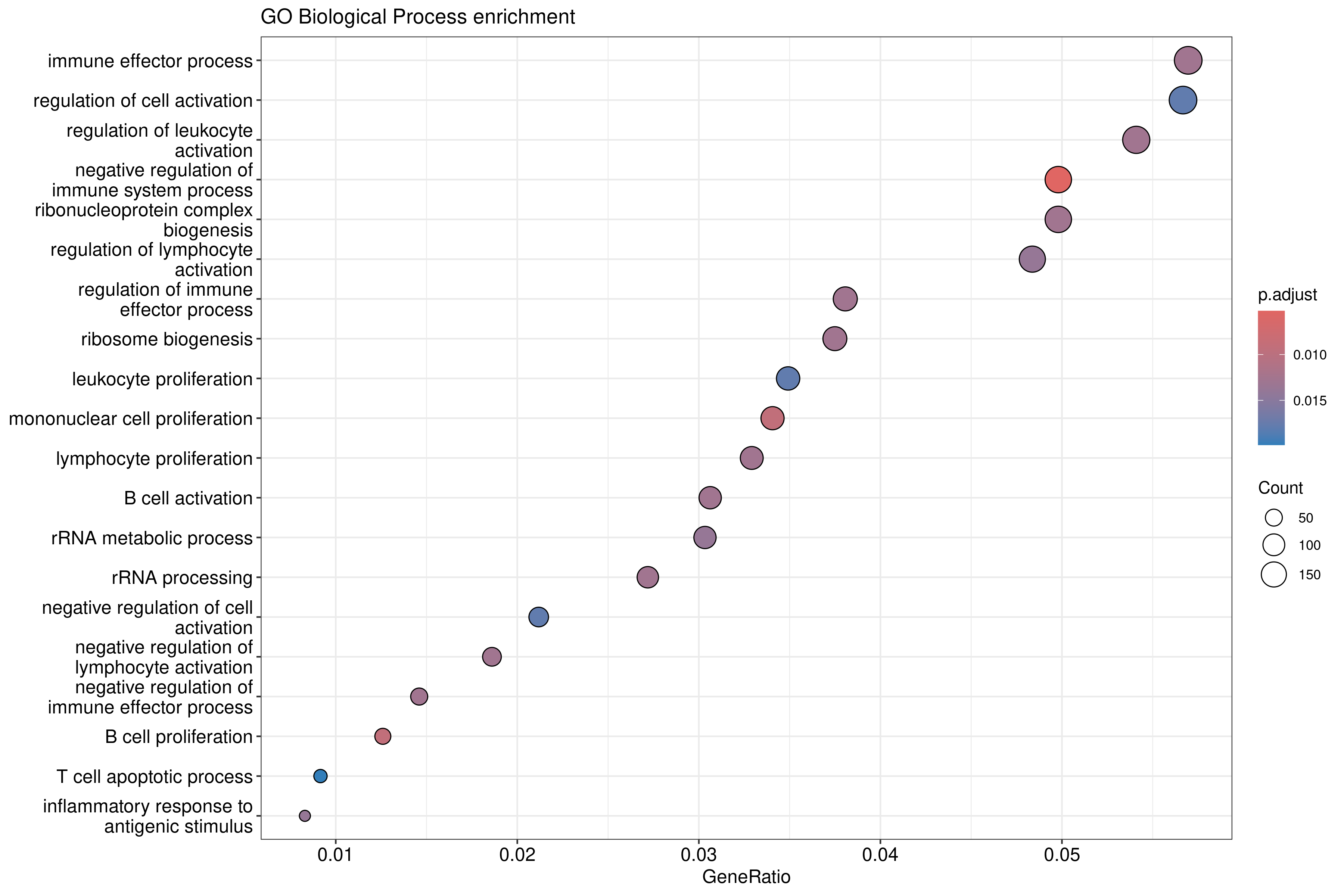
The dotplot shows: - X-axis: Gene ratio (proportion of DE genes in the term) - Y-axis: GO term description - Color: Adjusted p-value - Size: Number of genes
Barplot alternative:
R
barplot(ego_bp, showCategory = 15) +
    ggtitle("GO BP enrichment - Top 15 terms")
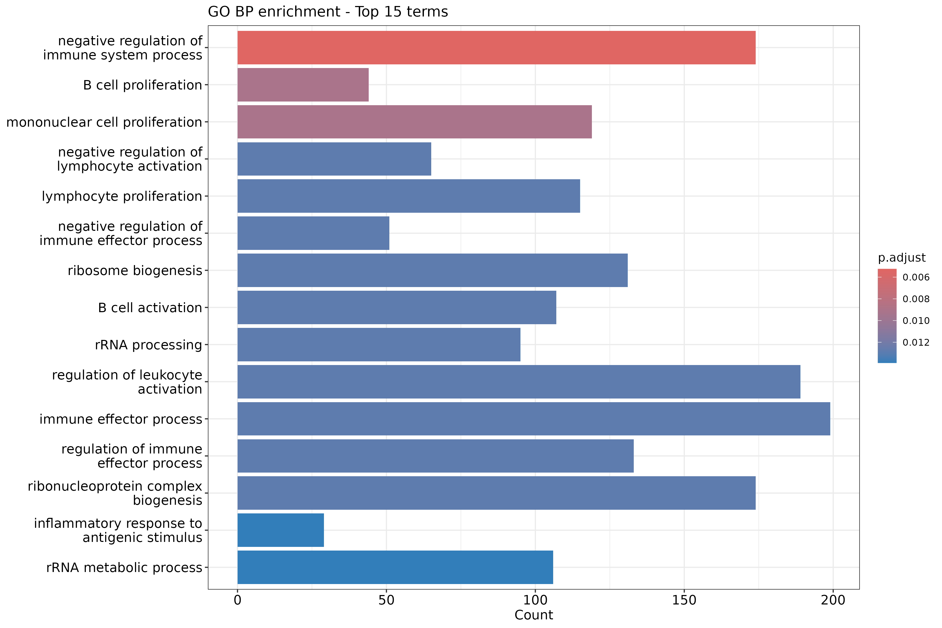
Reduce GO redundancy
GO terms are hierarchical and often redundant. Use
simplify() to remove similar terms:
R
ego_bp_simple <- simplify(
    ego_bp,
    cutoff = 0.7,
    by = "p.adjust",
    select_fun = min
)

dotplot(ego_bp_simple, showCategory = 15) +
    ggtitle("GO BP enrichment (simplified)")
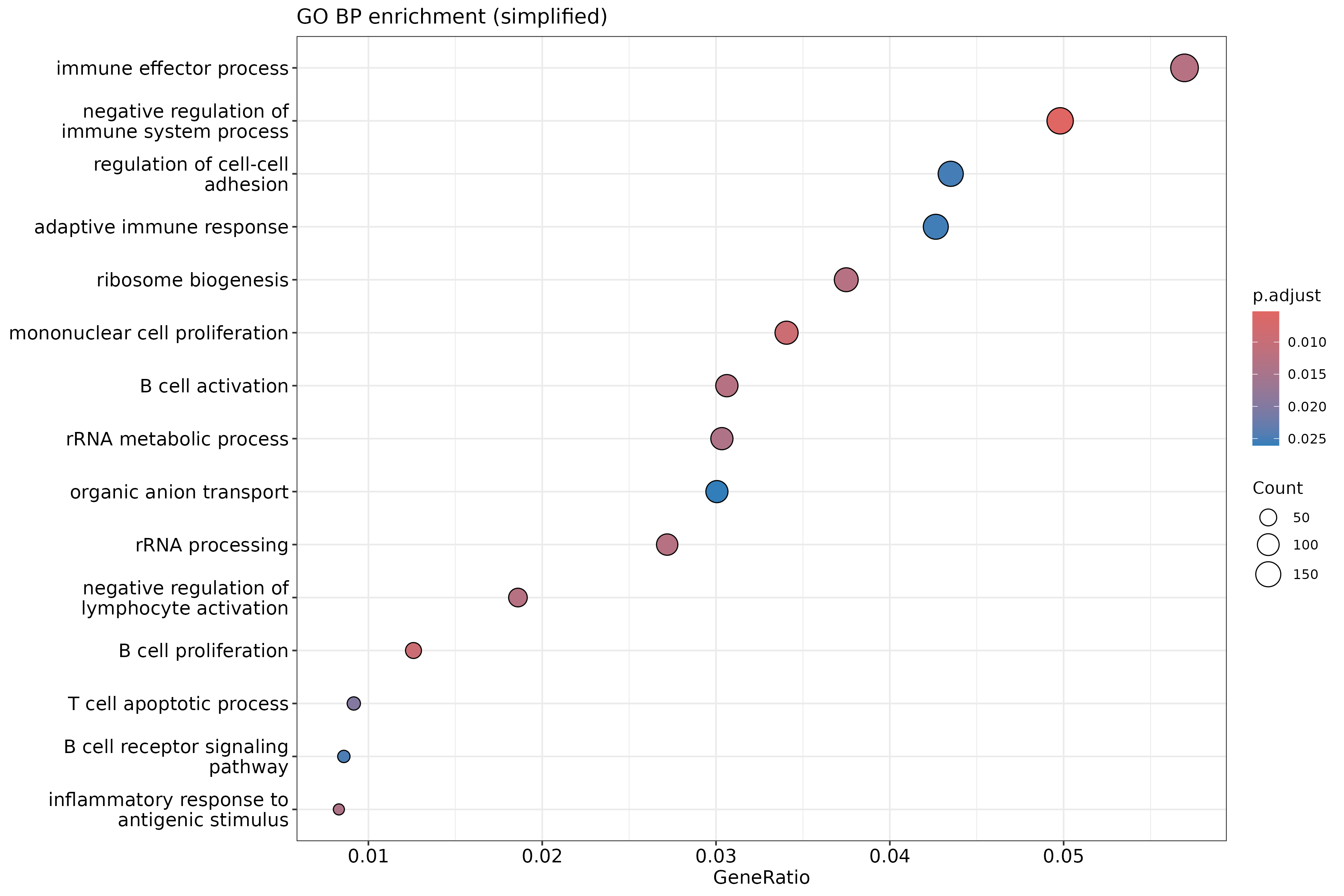
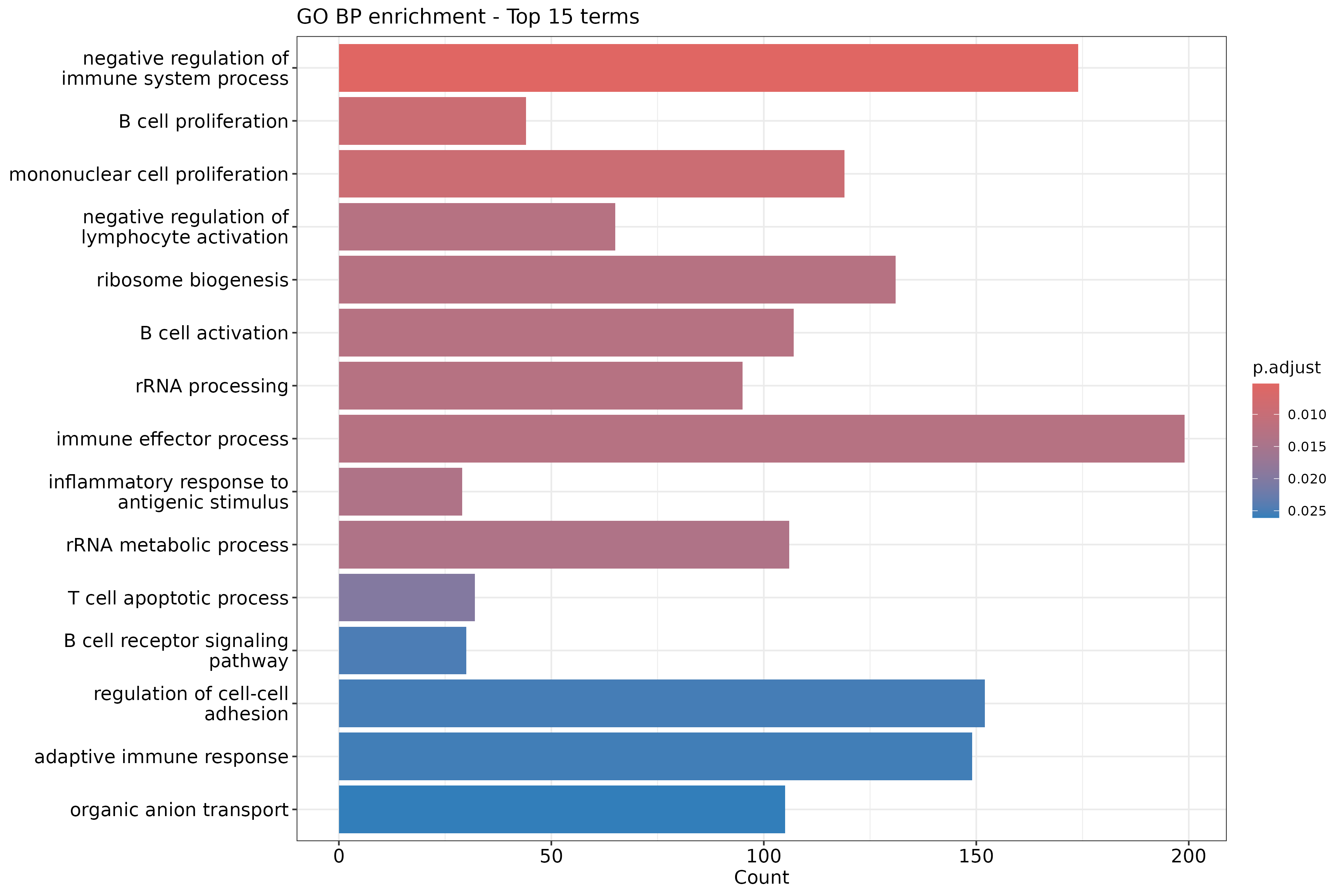
Why simplify GO results?
The GO hierarchy means related terms often appear together: - “regulation of cell death” and “positive regulation of cell death” - “response to stimulus” and “response to external stimulus”
simplify() removes redundant terms based on semantic
similarity, making results easier to interpret. The cutoff
parameter (0-1) controls how aggressively terms are merged.
Enrichment map visualization
For many significant terms, an enrichment map shows relationships:
R
ego_bp_em <- pairwise_termsim(ego_bp_simple)
emapplot(ego_bp_em, showCategory = 30) +
    ggtitle("GO BP enrichment map")
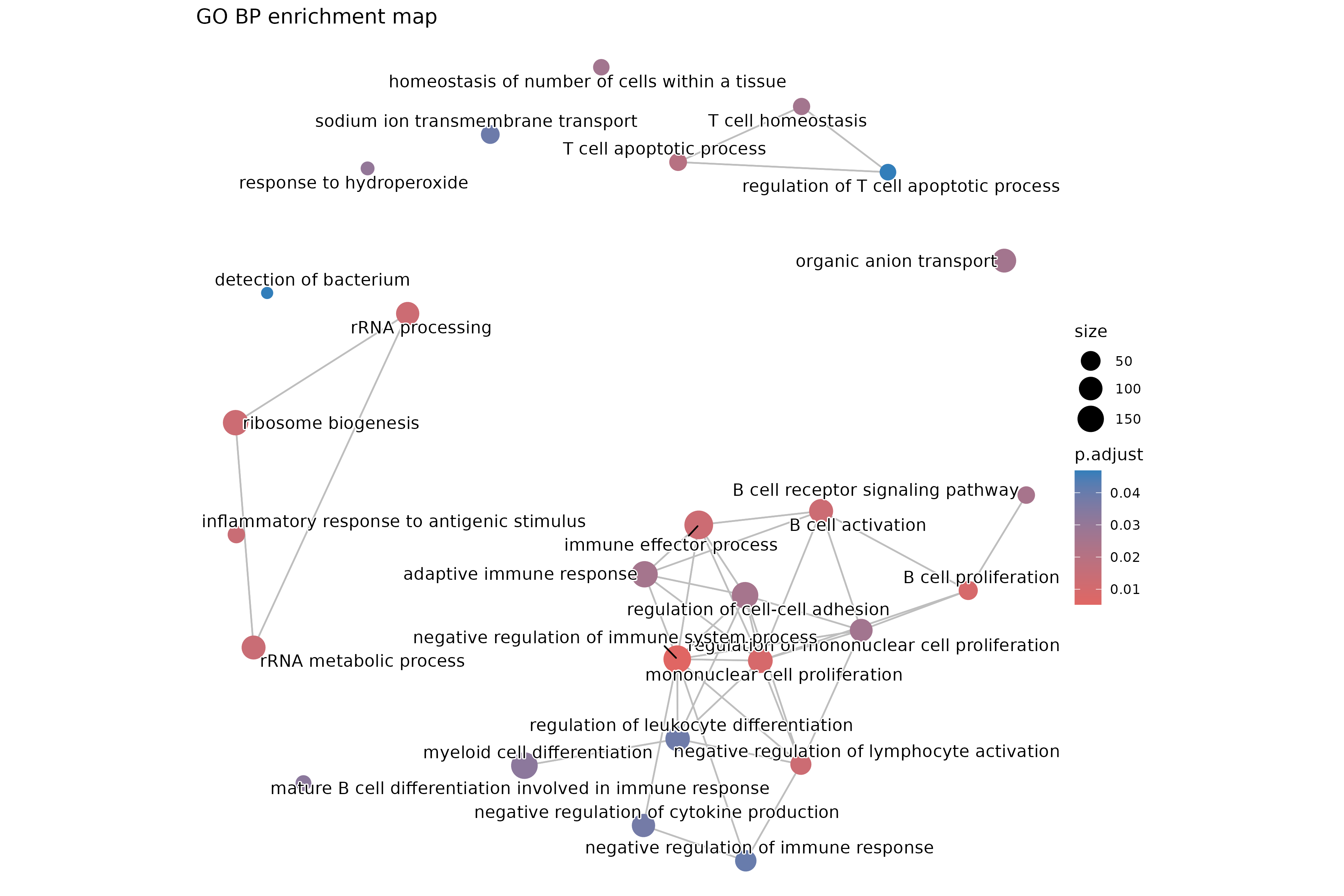
The enrichment map clusters similar terms together, revealing functional themes.
Exercise: Compare GO ontologies
Run enrichment for GO Molecular Function (MF) and Cellular Component (CC):
R
ego_mf <- enrichGO(gene = sig_entrez, universe = universe_entrez,
                   OrgDb = org.Mm.eg.db, ont = "MF", readable = TRUE)
ego_cc <- enrichGO(gene = sig_entrez, universe = universe_entrez,
                   OrgDb = org.Mm.eg.db, ont = "CC", readable = TRUE)
- How do the top terms differ between BP, MF, and CC?
- Are there consistent themes across ontologies?
- Which ontology provides the most interpretable results for your experiment?
Example interpretation:
- BP terms describe processes (e.g., “cell cycle”, “RNA processing”).
- MF terms describe molecular activities (e.g., “RNA binding”, “kinase activity”).
- CC terms describe locations (e.g., “nucleus”, “mitochondrion”).
Consistent themes across ontologies strengthen biological interpretation. For example, if BP shows “translation” enrichment, MF might show “ribosome binding”, and CC might show “ribosome” or “cytoplasm”.
Step 3: KEGG pathway enrichment
KEGG provides curated pathway maps connecting genes to biological systems.
R
ekegg <- enrichKEGG(
    gene = sig_entrez,
    universe = universe_entrez,
    organism = "mmu",  # Mouse
    pAdjustMethod = "BH",
    pvalueCutoff = 0.05
)

head(ekegg)
Output (geneID column not shown for brevity):
                                    category                         subcategory       ID                              Description GeneRatio BgRatio RichFactor
mmu04115                   Cellular Processes               Cell growth and death mmu04115                    p53 signaling pathway   41/1686 64/5208  0.6406250
mmu05322                       Human Diseases                      Immune disease mmu05322             Systemic lupus erythematosus   46/1686 87/5208  0.5287356
mmu04977                   Organismal Systems                    Digestive system mmu04977         Vitamin digestion and absorption   12/1686 15/5208  0.8000000
mmu04514 Environmental Information Processing Signaling molecules and interaction mmu04514 Cell adhesion molecule (CAM) interaction   43/1686 85/5208  0.5058824
mmu05150                       Human Diseases       Infectious disease: bacterial mmu05150          Staphylococcus aureus infection   19/1686 30/5208  0.6333333
mmu04981                                 <NA>                                <NA> mmu04981          Folate transport and metabolism   13/1686 18/5208  0.7222222
         FoldEnrichment   zScore       pvalue     p.adjust       qvalue
mmu04115       1.978870 5.451204 1.688415e-07 5.605537e-05 5.491791e-05
mmu05322       1.633247 4.120819 5.329885e-05 8.847610e-03 8.668077e-03
mmu04977       2.471174 3.947558 2.042589e-04 2.260466e-02 2.214597e-02
mmu04514       1.562654 3.618403 3.393132e-04 2.816300e-02 2.759152e-02
mmu05150       1.956346 3.634316 4.705801e-04 3.124652e-02 3.061248e-02
mmu04981       2.230921 3.619185 6.082405e-04 3.365597e-02 3.297304e-02
         Count
mmu04115    41
mmu05322    46
mmu04977    12
mmu04514    43
mmu05150    19
mmu04981 13KEGG organism codes
Common organism codes: - "hsa": Human -
"mmu": Mouse - "rno": Rat -
"dme": Drosophila - "sce": Yeast -
"ath": Arabidopsis
Find your organism:
search_kegg_organism("species name")
Visualize KEGG results:
R
barplot(ekegg, showCategory = 15) +
    ggtitle("KEGG pathway enrichment")
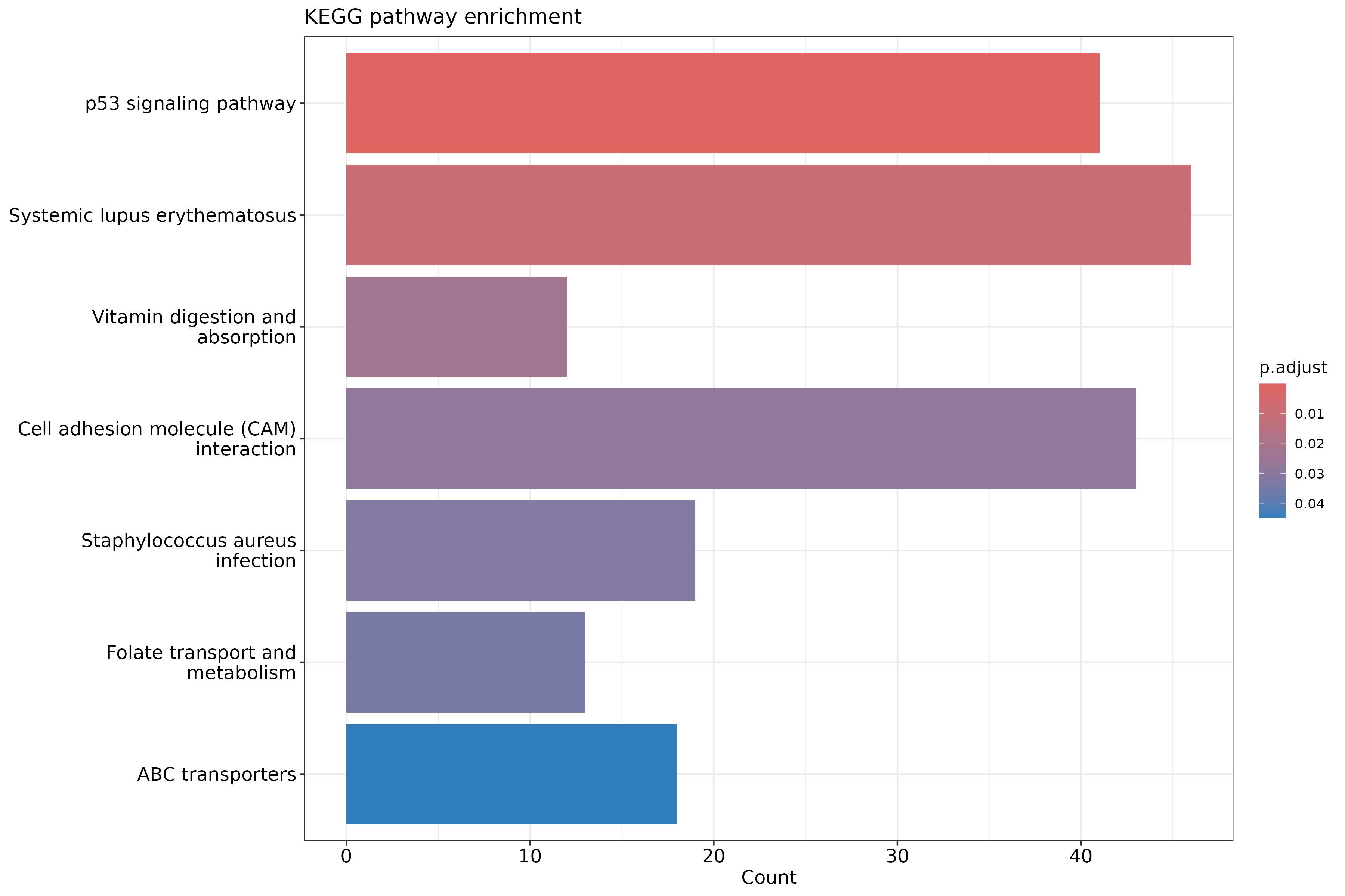
KEGG limitations
Be aware of KEGG-specific issues:
- ID coverage: KEGG uses its own gene IDs; some Entrez IDs may not map.
- Update frequency: KEGG pathways are updated periodically; results may vary.
- License: KEGG has usage restrictions for commercial applications.
- Incomplete mapping: Some genes lack pathway assignments.
Check dropped genes:
R
message(sprintf("KEGG analysis used %d of %d input genes",
    length(ekegg@gene), length(sig_entrez)))
Output:
KEGG analysis used 3607 of 3608 input genesStep 4: MSigDB Hallmark enrichment
MSigDB Hallmark gene sets are 50 curated signatures representing well-defined biological states and processes.
Load Hallmark gene sets
R
hallmark <- msigdbr(species = "Mus musculus", category = "H")
head(hallmark)
Output:
# A tibble: 6 × 26
  gene_symbol ncbi_gene ensembl_gene       db_gene_symbol db_ncbi_gene db_ensembl_gene source_gene gs_id gs_name  gs_collection gs_subcollection gs_collection_name
  <chr>       <chr>     <chr>              <chr>          <chr>        <chr>           <chr>       <chr> <chr>    <chr>         <chr>            <chr>
1 Abca1       11303     ENSMUSG00000015243 ABCA1          19           ENSG00000165029 ABCA1       M5905 HALLMAR… H             ""               Hallmark
2 Abcb8       74610     ENSMUSG00000028973 ABCB8          11194        ENSG00000197150 ABCB8       M5905 HALLMAR… H             ""               Hallmark
3 Acaa2       52538     ENSMUSG00000036880 ACAA2          10449        ENSG00000167315 ACAA2       M5905 HALLMAR… H             ""               Hallmark
4 Acadl       11363     ENSMUSG00000026003 ACADL          33           ENSG00000115361 ACADL       M5905 HALLMAR… H             ""               Hallmark
5 Acadm       11364     ENSMUSG00000062908 ACADM          34           ENSG00000117054 ACADM       M5905 HALLMAR… H             ""               Hallmark
6 Acads       11409     ENSMUSG00000029545 ACADS          35           ENSG00000122971 ACADS       M5905 HALLMAR… H             ""               Hallmark
# ℹ 14 more variables: gs_description <chr>, gs_source_species <chr>, gs_pmid <chr>, gs_geoid <chr>, gs_exact_source <chr>, gs_url <chr>, db_version <chr>,
#   db_target_species <chr>, ortholog_taxon_id <int>, ortholog_sources <chr>, num_ortholog_sources <dbl>, entrez_gene <chr>, gs_cat <chr>, gs_subcat <chr>
Prepare gene set list:
R
hallmark_list <- hallmark %>%
    dplyr::select(gs_name, entrez_gene) %>%
    dplyr::rename(term = gs_name, gene = entrez_gene)
Run Hallmark enrichment
R
ehall <- enricher(
    gene = sig_entrez,
    universe = universe_entrez,
    TERM2GENE = hallmark_list,
    pAdjustMethod = "BH",
    pvalueCutoff = 0.05
)

head(ehall)
Output (columns truncated for brevity):
                                             ID             Description GeneRatio  BgRatio RichFactor FoldEnrichment   zScore       pvalue     p.adjust
HALLMARK_MYC_TARGETS_V2 HALLMARK_MYC_TARGETS_V2 HALLMARK_MYC_TARGETS_V2   40/1134  57/3216  0.7017544       1.990161 5.565765 6.573980e-08 3.286990e-06
HALLMARK_P53_PATHWAY       HALLMARK_P53_PATHWAY    HALLMARK_P53_PATHWAY   86/1134 164/3216  0.5243902       1.487160 4.725607 2.814573e-06 7.036433e-05
Visualize:
R
dotplot(ehall, showCategory = 20) +
    ggtitle("MSigDB Hallmark enrichment")
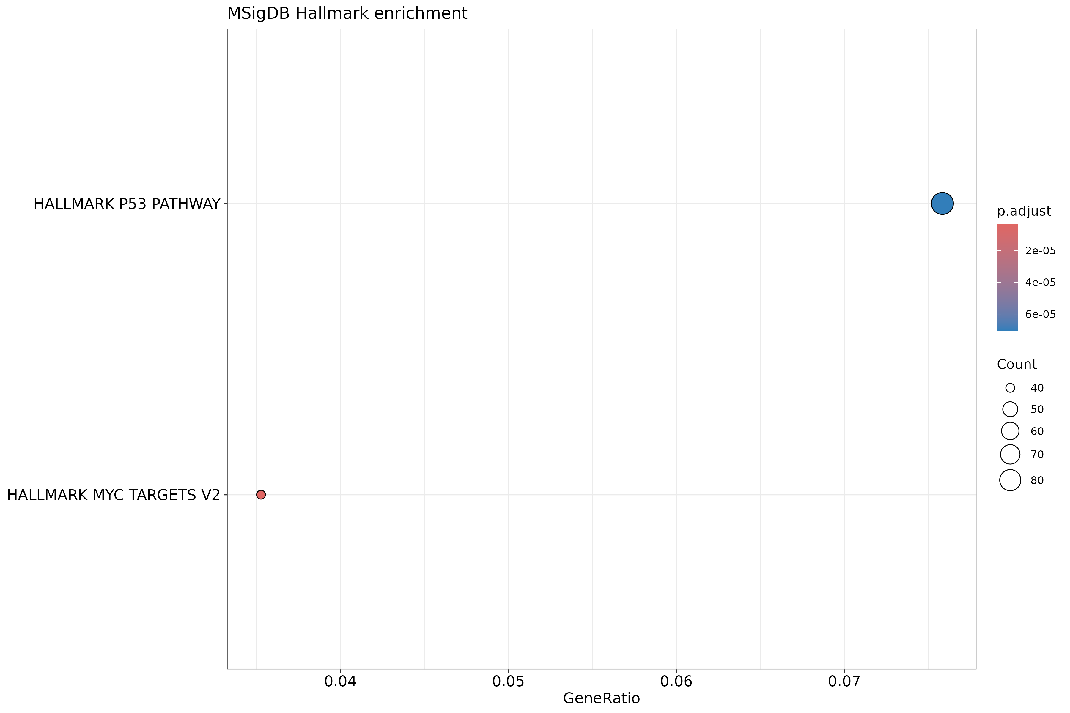
Why use Hallmark gene sets?
Advantages of Hallmark over GO/KEGG:
- Reduced redundancy: Each signature is distinct and non-overlapping.
- Expert curation: Refined from multiple sources to represent coherent biology.
- Interpretability: 50 sets is manageable for detailed examination.
- Reproducibility: Well-documented and stable definitions.
Common Hallmark sets include: - HALLMARK_INFLAMMATORY_RESPONSE - HALLMARK_P53_PATHWAY - HALLMARK_OXIDATIVE_PHOSPHORYLATION - HALLMARK_MYC_TARGETS_V1
Step 5: Compare results across databases
Create a summary of top enriched terms from each database:
R
# Extract top 10 from each
top_go <- head(ego_bp_simple@result, 10) %>%
    mutate(Database = "GO BP") %>%
    dplyr::select(Database, Description, p.adjust, Count)

top_kegg <- head(ekegg@result, 10) %>%
    mutate(Database = "KEGG") %>%
    dplyr::select(Database, Description, p.adjust, Count)

top_hall <- head(ehall@result, 10) %>%
    mutate(Database = "Hallmark") %>%
    dplyr::select(Database, ID, p.adjust, Count) %>%
    dplyr::rename(Description = ID)

# Combine
comparison <- bind_rows(top_go, top_kegg, top_hall)
comparison
Output:
                                 Database                                  Description     p.adjust Count
GO:0002683                          GO BP negative regulation of immune system process 5.247415e-03   174
GO:0042100                          GO BP                         B cell proliferation 9.166217e-03    44
GO:0032943                          GO BP               mononuclear cell proliferation 9.166217e-03   119
GO:0051250                          GO BP negative regulation of lymphocyte activation 1.278238e-02    65
GO:0042254                          GO BP                          ribosome biogenesis 1.278238e-02   131
GO:0042113                          GO BP                            B cell activation 1.278238e-02   107
GO:0006364                          GO BP                              rRNA processing 1.278238e-02    95
GO:0002252                          GO BP                      immune effector process 1.278238e-02   199
GO:0002437                          GO BP  inflammatory response to antigenic stimulus 1.390022e-02    29
GO:0016072                          GO BP                       rRNA metabolic process 1.390022e-02   106
mmu04115                             KEGG                        p53 signaling pathway 5.605537e-05    41
mmu05322                             KEGG                 Systemic lupus erythematosus 8.847610e-03    46
mmu04977                             KEGG             Vitamin digestion and absorption 2.260466e-02    12
mmu04514                             KEGG     Cell adhesion molecule (CAM) interaction 2.816300e-02    43
mmu05150                             KEGG              Staphylococcus aureus infection 3.124652e-02    19
mmu04981                             KEGG              Folate transport and metabolism 3.365597e-02    13
mmu02010                             KEGG                             ABC transporters 4.462944e-02    18
mmu03008                             KEGG            Ribosome biogenesis in eukaryotes 8.758267e-02    35
mmu05202                             KEGG      Transcriptional misregulation in cancer 9.020508e-02    60
mmu04068                             KEGG                       FoxO signaling pathway 1.135249e-01    48
HALLMARK_MYC_TARGETS_V2          Hallmark                      HALLMARK_MYC_TARGETS_V2 3.286990e-06    40
HALLMARK_P53_PATHWAY             Hallmark                         HALLMARK_P53_PATHWAY 7.036433e-05    86
HALLMARK_XENOBIOTIC_METABOLISM   Hallmark               HALLMARK_XENOBIOTIC_METABOLISM 1.034831e-01    57
HALLMARK_HEME_METABOLISM         Hallmark                     HALLMARK_HEME_METABOLISM 1.034831e-01    72
HALLMARK_IL2_STAT5_SIGNALING     Hallmark                 HALLMARK_IL2_STAT5_SIGNALING 1.611589e-01    69
HALLMARK_ALLOGRAFT_REJECTION     Hallmark                 HALLMARK_ALLOGRAFT_REJECTION 1.611589e-01    70
HALLMARK_MYC_TARGETS_V1          Hallmark                      HALLMARK_MYC_TARGETS_V1 1.757524e-01    84
HALLMARK_TNFA_SIGNALING_VIA_NFKB Hallmark             HALLMARK_TNFA_SIGNALING_VIA_NFKB 2.021817e-01    67
HALLMARK_ESTROGEN_RESPONSE_EARLY Hallmark             HALLMARK_ESTROGEN_RESPONSE_EARLY 2.021817e-01    56
HALLMARK_APOPTOSIS Hallmark HALLMARK_APOPTOSIS 2.527274e-01 54Exercise: Identify convergent themes
Looking at your GO, KEGG, and Hallmark results:
- Are there biological themes that appear across multiple databases?
- Are there database-specific findings that don’t replicate elsewhere?
- How would you prioritize which findings to investigate further?
Convergent signals to look for:
- If GO shows “cell cycle” terms, KEGG might show “Cell cycle” pathway, and Hallmark might show “HALLMARK_G2M_CHECKPOINT”.
- If GO shows “immune response”, KEGG might show “Cytokine-cytokine receptor interaction”, and Hallmark might show “HALLMARK_INFLAMMATORY_RESPONSE”.
Database-specific findings may indicate: - Pathway coverage differences. - Annotation biases. - Potentially spurious signals (require validation).
Prioritization strategy: 1. Focus on themes appearing in multiple databases. 2. Consider effect size (how many genes, fold enrichment). 3. Assess biological plausibility given experimental design. 4. Validate key findings with independent methods.
Step 5b: Direction-aware enrichment analysis
ORA on all significant genes (up + down combined) can mask biological signals when up-regulated and down-regulated genes have different functions. Analyzing directions separately often reveals clearer patterns.
Prepare direction-specific gene lists
R
# Up-regulated genes
up_genes <- res %>%
    filter(padj < 0.05, log2FoldChange > log2fc_cut) %>%
    pull(ensembl_gene_id_version)
up_clean <- gsub("\\.\\d+$", "", up_genes)
up_entrez <- id_map %>%
    filter(ENSEMBL %in% up_clean) %>%
    pull(ENTREZID)

# Down-regulated genes
down_genes <- res %>%
    filter(padj < 0.05, log2FoldChange < -log2fc_cut) %>%
    pull(ensembl_gene_id_version)
down_clean <- gsub("\\.\\d+$", "", down_genes)
down_entrez <- id_map %>%
    filter(ENSEMBL %in% down_clean) %>%
    pull(ENTREZID)

message(sprintf("Up-regulated: %d genes, Down-regulated: %d genes",
    length(up_entrez), length(down_entrez)))
Up-regulated: 1810 genes, Down-regulated: 1798 genesRun enrichment for each direction
R
# GO enrichment for up-regulated genes
ego_up <- enrichGO(
    gene = up_entrez,
    universe = universe_entrez,
    OrgDb = org.Mm.eg.db,
    ont = "BP",
    readable = TRUE
)

# GO enrichment for down-regulated genes
ego_down <- enrichGO(
    gene = down_entrez,
    universe = universe_entrez,
    OrgDb = org.Mm.eg.db,
    ont = "BP",
    readable = TRUE
)
Compare directions
R
# Combine top results for comparison
up_top <- head(ego_up@result, 10) %>%
    mutate(Direction = "Up-regulated") %>%
    dplyr::select(Direction, Description, p.adjust, Count)

down_top <- head(ego_down@result, 10) %>%
    mutate(Direction = "Down-regulated") %>%
    dplyr::select(Direction, Description, p.adjust, Count)

direction_comparison <- bind_rows(up_top, down_top)
direction_comparison
Output:
                Direction                                                                              Description     p.adjust Count
GO:0002694   Up-regulated                                                       regulation of leukocyte activation 7.705961e-07   127
GO:0002683   Up-regulated                                             negative regulation of immune system process 9.130747e-07   113
GO:0050865   Up-regulated                                                            regulation of cell activation 1.389200e-06   131
GO:0002252   Up-regulated                                                                  immune effector process 1.389200e-06   130
GO:0007264   Up-regulated                                                small GTPase-mediated signal transduction 2.781020e-06    95
GO:0051249   Up-regulated                                                      regulation of lymphocyte activation 4.543747e-06   111
GO:0009617   Up-regulated                                                                    response to bacterium 4.720694e-06   120
GO:0002697   Up-regulated                                                    regulation of immune effector process 1.175944e-05    88
GO:0007186   Up-regulated                                             G protein-coupled receptor signaling pathway 1.175944e-05    97
GO:0030036   Up-regulated                                                          actin cytoskeleton organization 3.108071e-05   123
GO:0022613 Down-regulated                                                     ribonucleoprotein complex biogenesis 2.154137e-27   164
GO:0042254 Down-regulated                                                                      ribosome biogenesis 3.115494e-25   128
GO:0006364 Down-regulated                                                                          rRNA processing 4.368810e-19    92
GO:0016072 Down-regulated                                                                   rRNA metabolic process 6.776964e-19   100
GO:0042273 Down-regulated                                                       ribosomal large subunit biogenesis 1.090959e-08    33
GO:0042274 Down-regulated                                                       ribosomal small subunit biogenesis 4.296891e-08    45
GO:0006399 Down-regulated                                                                   tRNA metabolic process 1.002785e-06    62
GO:0000470 Down-regulated                                                                   maturation of LSU-rRNA 2.496138e-05    17
GO:0009451 Down-regulated                                                                         RNA modification 4.970122e-05    48
GO:0000463 Down-regulated maturation of LSU-rRNA from tricistronic rRNA transcript (SSU-rRNA, 5.8S rRNA, LSU-rRNA) 7.457449e-05 13When to analyze directions separately
Separate analysis is particularly useful when:
- You expect different biological processes to be activated vs. suppressed.
- Combined analysis shows few significant results (opposing signals may cancel out).
- You want to understand mechanism (what’s gained vs. lost).
Separate analysis is less useful when:
- You have very few DE genes in one direction.
- The biological question is about overall pathway disruption.
Step 5c: Gene Set Enrichment Analysis (GSEA)
ORA has a fundamental limitation: it requires an arbitrary cutoff to define “significant” genes. GSEA uses the full ranked gene list without cutoffs.
How GSEA differs from ORA
| Aspect | ORA | GSEA |
|---|---|---|
| Input | List of significant genes | All genes, ranked by fold change |
| Cutoff | Required (padj, LFC) | None |
| Sensitivity | May miss coordinated small changes | Detects subtle but consistent shifts |
| Gene weights | All DE genes treated equally | Magnitude of change matters |
Prepare ranked gene list for GSEA
GSEA requires a named vector of gene scores (typically log2 fold change or a signed significance score):
R
# Create ranked list using signed -log10(pvalue) * sign(LFC)
# This weights by both significance and direction
res_gsea <- res %>%
    filter(!is.na(padj), !is.na(log2FoldChange)) %>%
    mutate(
        ensembl_clean = gsub("\\.\\d+$", "", ensembl_gene_id_version),
        rank_score = -log10(pvalue) * sign(log2FoldChange)
    )

# Map to Entrez IDs
res_gsea <- res_gsea %>%
    inner_join(id_map, by = c("ensembl_clean" = "ENSEMBL"))

# Create named vector (required format for GSEA)
gene_list <- res_gsea$rank_score
names(gene_list) <- res_gsea$ENTREZID

# Sort by rank score (required for GSEA)
gene_list <- sort(gene_list, decreasing = TRUE)
Run GSEA with clusterProfiler
R
# 1. Sort the list in decreasing order (required by clusterProfiler)
gene_list <- sort(gene_list, decreasing = TRUE)
# 2. Remove duplicate Entrez IDs
# (Since we sorted by value, this keeps the instance with the highest absolute value)
gene_list <- gene_list[!duplicated(names(gene_list))]
# 3. Verify it is a numeric vector
# (It should look like: 261.1, 126.5... with names "20343", "108105"...)
head(gene_list)
# 4. Run GSEA
gsea_go <- gseGO(
    geneList     = gene_list,      # Pass the numeric vector, NOT names(gene_list)
    OrgDb        = org.Mm.eg.db,
    ont          = "BP",
    minGSSize    = 10,
    maxGSSize    = 500,
    pvalueCutoff = 0.05,
    verbose      = FALSE
)
head(gsea_go)
Output (columns truncated for brevity):
                   ID                                   Description setSize enrichmentScore       NES       pvalue     p.adjust       qvalue rank
GO:0042254 GO:0042254                           ribosome biogenesis     304      -0.7713857 -2.022231 1.000000e-10 0.0000001312 1.169211e-07 1867
GO:0006364 GO:0006364                               rRNA processing     210      -0.7694754 -1.950534 1.000000e-10 0.0000001312 1.169211e-07 1867
GO:0016072 GO:0016072                        rRNA metabolic process     241      -0.7525383 -1.933838 1.000000e-10 0.0000001312 1.169211e-07 1867
GO:0022613 GO:0022613          ribonucleoprotein complex biogenesis     425      -0.7186644 -1.919595 1.000000e-10 0.0000001312 1.169211e-07 1867
GO:0042770 GO:0042770 signal transduction in response to DNA damage     170      -0.7420666 -1.849975 1.315390e-07 0.0001380633 1.230374e-04  892
GO:0042274 GO:0042274            ribosomal small subunit biogenesis     106      -0.7953618 -1.887333 2.644409e-07 0.0002312976 2.061247e-04  948
Visualize GSEA results
R
# Dot plot of enriched gene sets
dotplot(gsea_go, showCategory = 20, split = ".sign") +
    facet_grid(. ~ .sign) +
    ggtitle("GSEA: GO Biological Process")
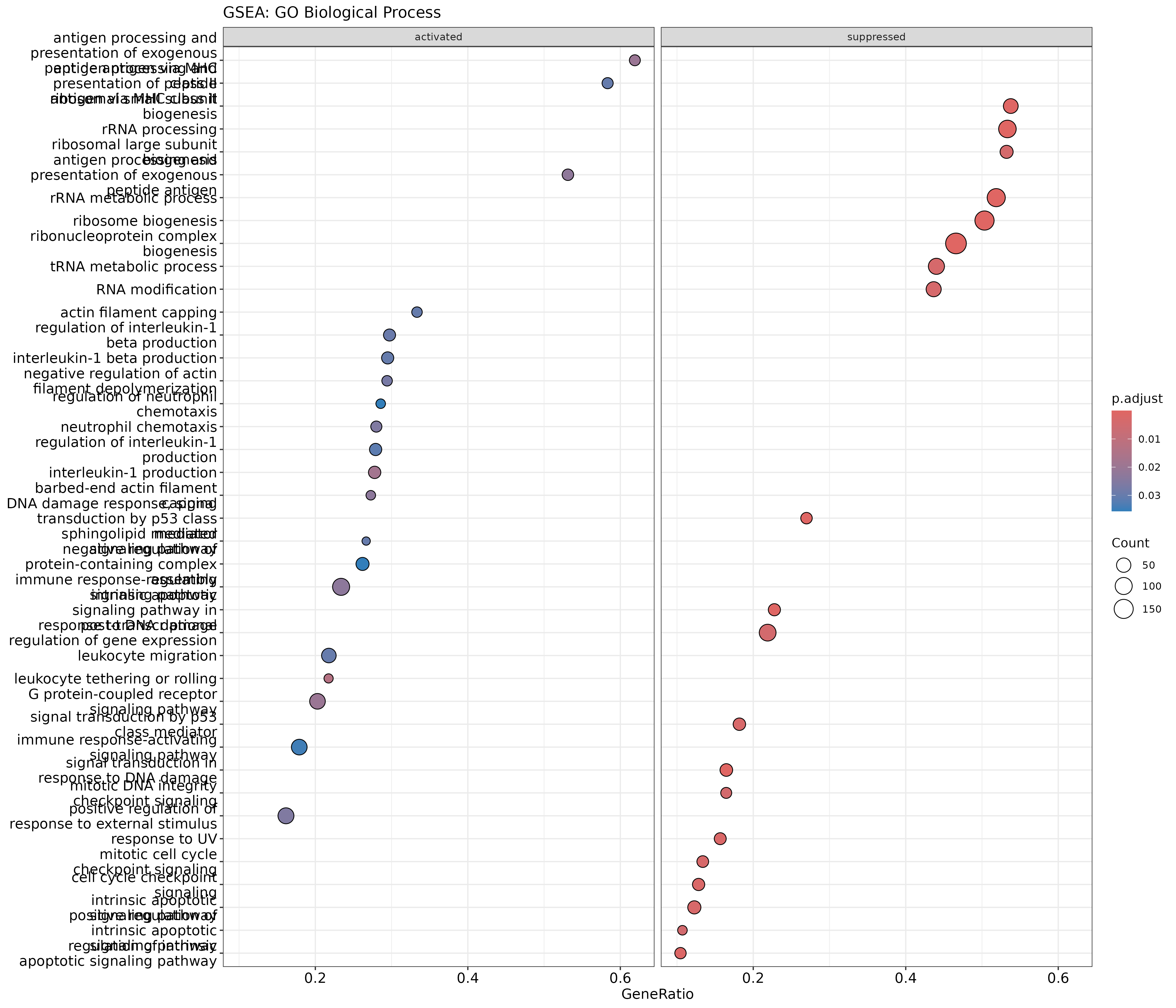
The .sign column indicates whether the gene set is
enriched in up-regulated (activated) or down-regulated
(suppressed) genes.
GSEA enrichment plot for a specific term
R
# Enrichment plot for top gene set
gseaplot2(gsea_go, geneSetID = 1, title = gsea_go$Description[1])
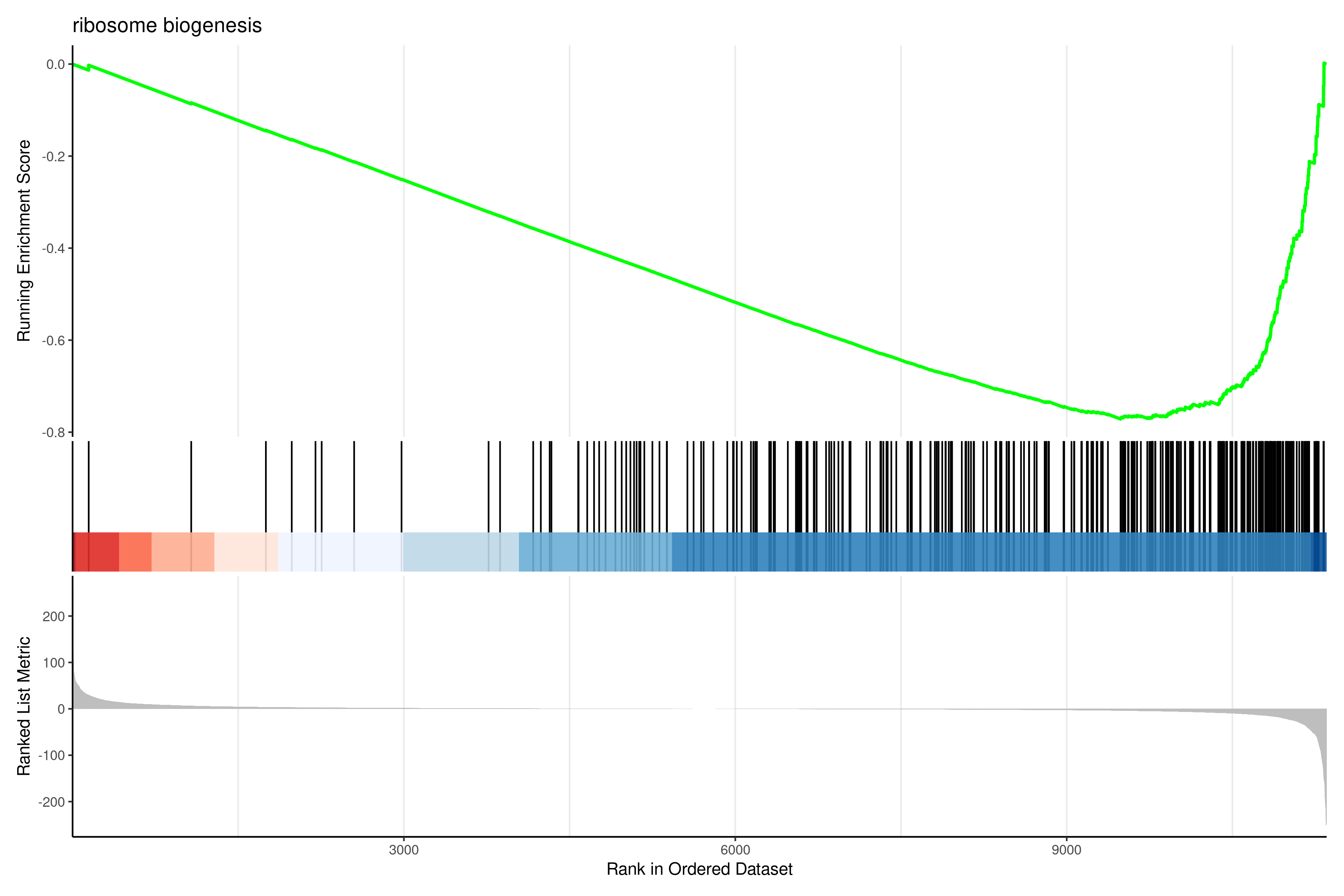
Interpreting GSEA results
Key metrics:
- NES (Normalized Enrichment Score): Direction and strength of enrichment. Positive = enriched in up-regulated genes; Negative = enriched in down-regulated genes.
- pvalue/p.adjust: Statistical significance.
- core_enrichment: Genes contributing most to the enrichment signal (“leading edge”).
GSEA is particularly valuable when:
- Changes are subtle but coordinated across many genes.
- You want to avoid arbitrary significance cutoffs.
- You’re comparing with published gene signatures.
Exercise: Compare ORA and GSEA results
- Do the same pathways appear in both ORA and GSEA results?
- Does GSEA identify any pathways that ORA missed?
- For pathways appearing in both, is the direction (NES sign) consistent with the ORA direction analysis?
Expected observations:
- Many top pathways should overlap between ORA and GSEA.
- GSEA may identify additional pathways where changes are subtle but coordinated.
- The NES sign (positive/negative) should match whether the pathway was enriched in up- or down-regulated genes in ORA.
- Discrepancies may indicate pathways where the signal comes from many small changes rather than a few large ones.
Step 6: Save results
Save all enrichment results:
R
# Create output directory
dir.create("results/enrichment", showWarnings = FALSE)

# GO results
write_csv(as.data.frame(ego_bp), "results/enrichment/GO_BP_enrichment.csv")
write_csv(as.data.frame(ego_bp_simple), "results/enrichment/GO_BP_simplified.csv")

# KEGG results
write_csv(as.data.frame(ekegg), "results/enrichment/KEGG_enrichment.csv")

# Hallmark results
write_csv(as.data.frame(ehall), "results/enrichment/Hallmark_enrichment.csv")

# Direction-aware results
write_csv(as.data.frame(ego_up), "results/enrichment/GO_BP_up_regulated.csv")
write_csv(as.data.frame(ego_down), "results/enrichment/GO_BP_down_regulated.csv")

# GSEA results
write_csv(as.data.frame(gsea_go), "results/enrichment/GSEA_GO_BP.csv")
Save plots:
R
# GO dotplot
pdf("results/enrichment/GO_BP_dotplot.pdf", width = 10, height = 8)
dotplot(ego_bp_simple, showCategory = 20) +
    ggtitle("GO Biological Process enrichment")
dev.off()

# KEGG barplot
pdf("results/enrichment/KEGG_barplot.pdf", width = 10, height = 6)
barplot(ekegg, showCategory = 15) +
    ggtitle("KEGG pathway enrichment")
dev.off()

# Hallmark dotplot
pdf("results/enrichment/Hallmark_dotplot.pdf", width = 10, height = 8)
dotplot(ehall, showCategory = 20) +
    ggtitle("MSigDB Hallmark enrichment")
dev.off()
Interpretation guidelines
Signs of meaningful enrichment
Enrichment results are more reliable when:
- Multiple related terms appear (not just one isolated hit).
- Consistent themes emerge across databases.
- Biological plausibility: Results align with known biology of your system.
- Reasonable gene counts: Terms with many genes (>5-10) are more robust.
- Moderate p-values: Extremely low p-values (e.g., 10^-50) may indicate annotation bias.
Common pitfalls
- Over-interpretation: A significant p-value doesn’t prove causation.
- Ignoring effect size: A term with 3/1000 genes is less meaningful than 30/100.
- Cherry-picking: Report all significant results, not just expected ones.
- Universe mismatch: Using wrong background inflates or deflates significance.
- Outdated annotations: Gene function annotations improve over time.
Summary
- ORA tests if gene sets contain more DE genes than expected by chance using the hypergeometric test.
- The background universe must include all genes that could have been detected as DE.
- Multiple testing correction (FDR) is essential when testing thousands of gene sets.
- GO provides comprehensive but redundant functional annotation; use
simplify()to reduce redundancy. - KEGG provides curated pathway maps but has limited gene coverage and requires Entrez IDs.
- MSigDB Hallmark sets offer 50 high-quality, non-redundant biological signatures.
- Direction-aware analysis (up vs. down separately) often reveals clearer biological signals.
- GSEA avoids arbitrary cutoffs by using the full ranked gene list; it detects subtle but coordinated changes.
- Convergent findings across multiple databases and methods strengthen biological interpretation.
- Always report methods, thresholds, and full results for reproducibility.