Content from Introduction to Genome assembly
Last updated on 2026-02-18 | Edit this page
Estimated time: 30 minutes
Overview
Questions
- What is genome assembly, and why is it important?
- What sequencing technologies can be used for genome assembly?
- What are de novo and reference-guided assemblies?
- What challenges arise when generating high-quality assemblies?
- What software tools are used for assembling genomes?
Objectives
- Learn key concepts and terminology related to genome assembly.
- Understand datasets and tools used for genome assembly.
- Describe major sequencing technologies and their impact on assembly.
- Identify common computational challenges in genome assembly.
- Explain fundamental strategies and algorithms used in genome assembly.
What is Genome Assembly?
Genome assembly is the process of reconstructing a complete genome sequence by arranging fragmented DNA sequences (reads) into a continuous sequence.
- Goal is to achieve a high-quality reference genome that accurately represents the structure and sequence of an organism’s DNA.
- It enables deeper understanding of genes, their function, and evolutionary history.
- Vital for studying complex traits, species diversity, and disease mechanisms.
Importance of Genome Assembly
- Applications in medicine, agriculture, conservation, and
biotechnology:
- Human genetics: Assembling genomes to identify disease-causing mutations.
- Crop improvement: Identifying beneficial traits in plant genomes.
- Conservation biology: Sequencing endangered species to understand genetic diversity.
- Examples of major genome sequencing projects (Human Genome Project, Vertebrate Genome Project).
De Novo vs. Reference-Guided Assembly
- De novo assembly:
- Used when no reference genome exists.
- Requires assembling the genome from scratch using computational methods.
- Example: Assembling a new plant species genome.
- Reference-guided assembly:
- Aligns reads to a closely related reference genome.
- Useful for identifying variations but limited by reference bias.
- Example: Human genome resequencing for variant detection.
Basic Steps in Genome Assembly
- Sequencing: Generating raw reads from a genome.
- Preprocessing & Quality Control: Filtering and trimming reads.
- Assembly: Aligning and merging overlapping reads into contigs.
- Scaffolding: Ordering contigs into larger scaffolds using long-range sequencing data or mapping techniques.
- Polishing: Correcting errors using additional data.
- Quality Assessment: Evaluating assembly completeness and accuracy.
- Downstream Analysis: Annotating genes, identifying variants, and studying genome structure.
Reference: doi:10.1016/j.xpro.2022.101506
Data types for Genome Assembly
Illumina
Excels at high-throughput, short-read sequencing with high accuracy.
Uses Sequencing-by-Synthesis (SBS). DNA is fragmented, adapters are attached, and the fragments are immobilized on a flowcell. A polymerase incorporates fluorescently labeled nucleotides, and a camera captures the emitted signals in real time. Each cycle represents one nucleotide added to the growing DNA strand.
PacBio HiFi
provide accurate long reads, balancing throughput and error correction.
Uses Single Molecule, Real-Time (SMRT) sequencing. DNA is ligated into circular molecules and loaded onto a chip with zero-mode waveguides (ZMWs). A polymerase synthesizes the complementary strand, incorporating fluorescently labeled nucleotides. The system detects light pulses in real time, capturing multiple passes of the same molecule to generate highly accurate HiFi reads.
Oxford Nanopore
enables ultra-long reads but requires more advanced error correction.
A single DNA strand is passed through a biological nanopore embedded in a membrane. As nucleotides move through the pore, they cause characteristic disruptions in an electrical current, which are interpreted by machine-learning algorithms to determine the sequence.
Challenges in Genome Assembly
- Repetitive Elements: Identical or similar sequences that occur multiple times in the genome, making it difficult to resolve unique regions.
- Heterozygosity: Presence of two or more alleles at a given locus, leading to ambiguous read alignments.
- Polyploidy: Multiple copies of chromosomes, complicating assembly due to similar sequences.
- Genome Size: Large genomes require more computational resources and specialized algorithms.
- Error Correction: Addressing sequencing errors and distinguishing true variants from artifacts.
- Structural Variants: Large-scale rearrangements, duplications, deletions, and inversions that disrupt contiguity.
Main programs used for Genome Assembly
- Data QC:
- NanoPlot: Visualization of sequencing data quality.
- FiltLong: Filtering long reads based on quality and length.
- Assembly:
- HiFiasm: HiFi assembler for PacBio data.
- Flye: de novo assembler for long reads.
- Post-processing:
- Medaka: Basecaller and consensus polishing for Flye assembly.
- Bionano Solve: Optical mapping for scaffolding and validation.
- Evaluation:
- QUAST: Quality assessment tool for evaluating assemblies.
- Compleasm (BUSCO alternative): Benchmarking tool for assessing genome completeness.
- Merqury: K-mer-based evaluation of assembly accuracy and completeness.
- Genome assembly reconstructs complete genome sequences from fragmented DNA reads.
- De novo assembly builds genomes without a reference, while reference-guided assembly uses existing genomes.
- Sequencing technologies like Illumina, PacBio HiFi, and Oxford Nanopore offer different read lengths and error rates.
- Challenges include repetitive elements, heterozygosity, and error correction.
- Tools many programs are available for data QC, assembly, post-processing, and evaluation - choice depends on data type and research goals.
Content from Assembly Strategies
Last updated on 2026-02-18 | Edit this page
Estimated time: 20 minutes
Overview
Questions
- What factors influence the choice of genome assembly strategy?
- How do different assembly methods compare in terms of read length, accuracy, and computational requirements?
- What are the key steps in evaluating genome assemblies using BUSCO and QUAST?
- How do Bionano OGM and Hi-C sequencing improve genome continuity and organization?
Objectives
- Understand factors influencing the choice of genome assembly strategy.
- Compare different assembly methods based on read length, accuracy, and computational requirements.
- Learn how to evaluate genome assemblies using BUSCO and QUAST.
- Explore the role of Bionano OGM and Hi-C sequencing in improving genome continuity.
Assembly Strategies
Genome assembly involves choosing the right approach based on sequencing technology, read type, genome complexity, and research objectives. This chapter introduces key factors influencing assembly strategy selection, from read length and coverage requirements to computational trade-offs. We will explore different methods—PacBio HiFi with HiFiasm, ONT with Flye, and hybrid assemblies—along with scaffolding techniques like Bionano Optical Genome Mapping (OGM) and Hi-C, which help improve genome continuity and organization. Finally, we’ll discuss assembly evaluation tools such as BUSCO and QUAST to assess the completeness and quality of assembled genomes.
Factors Influencing the Choice of Strategy
-
Read length: Affects the ability to resolve
repeats; short reads struggle with complex regions, while long reads
improve contiguity.
-
Coverage depth: Crucial for assembly accuracy, with
HiFi requiring 20-30x, ONT needing 50-100x, and hybrid assemblies
depending on short-read support for polishing.
-
Genome complexity: Includes repeat content,
heterozygosity, and polyploidy, which influence assembly success and
determine whether specialized tools or additional scaffolding methods
are needed.
-
Computational resources: Vary across assembly
strategies, with HiFiasm being RAM-intensive, Flye being more
lightweight, and hybrid assemblies requiring additional processing for
polishing.
-
Sequencing budget: Plays a role, as HiFi sequencing
is costlier but highly accurate, ONT is cheaper but requires more data
for error correction, and hybrid approaches balance cost and
quality.
- Downstream analyses: Structural variation detection, gene annotation, or chromosome-level assemblies influence the choice of assembler and the need for scaffolding methods like Hi-C or Bionano OGM.
Comparative Assembly Strategies
| Factor | PacBio HiFi | ONT | Hybrid (ONT + PacBio HiFi) |
|---|---|---|---|
| Read length | ~15-20kb | 10-100kb+ | Mix of ultra-long & accurate |
| Read accuracy | High (~99%) | Variable: ~90% (R9/fast) to ~99% (R10.4/HAC/SUP) | High (after polishing) |
| Coverage needed | 20-30x | 50-100x | ONT: 50x + HiFi: 20-30x |
| Cost per Gb | Expensive | Lower | Medium |
| Error profile | Random errors, low indels | Systematic errors in homopolymers; greatly reduced with R10.4+ | ONT errors corrected by HiFi reads |
| Computational requirements | High RAM required | Moderate RAM required | Moderate |
| Best for | High-accuracy assemblies | Ultra-long contigs | Combines advantages of both |
| Repeat resolution | Good | Very good | Very good |
| Scaffolding needed | Rarely needed | May be needed | Sometimes needed |
| Polishing required | Not required | Required (Medaka) | Polish with HiFi reads |
| Structural variant detection | Good | Excellent | Good |
| Haplotype phasing | Excellent | Good | Moderate |
| Genome size suitability | Suitable for large and small genomes | Best for large genomes | Best for complex genomes |
| Downstream applications | Reference-quality genome assembly, annotation | Structural variation analysis, de novo assembly | Genome correction, variant calling, scaffolding |
Contig vs. Scaffold vs. Chromosome-Level Assembly
Genome assemblies progress through different levels of completeness and organization:
-
Contig-level assembly: The raw output of
assemblers, consisting of contiguous sequences without known order or
orientation. Longer contigs indicate better assembly continuity.
-
Scaffold-level assembly: Contigs linked together
using additional data (e.g., long-range mate-pair reads, optical maps,
or Hi-C). Gaps (represented as ’N’s) remain where connections exist but
sequence information is missing.
- Chromosome-level assembly: The highest-quality assembly, where scaffolds are further ordered and oriented into full chromosomes using genetic maps, Hi-C data, or synteny with a reference genome.
Higher levels of assembly provide better genome context, but require additional scaffolding methods beyond de novo assembly.
Workflow for Various Assemblies
In this workshop, we will use HiFiasm for PacBio HiFi assemblies, Flye for ONT assemblies, and Flye in hybrid mode for ONT + PacBio HiFi assemblies, followed by quality assessment using Compleasm and QUAST to evaluate completeness and accuracy.
PacBio HiFi Assembly with HiFiasm
- PacBio HiFi reads: Highly accurate long reads with low error rates, suitable for de novo assembly without polishing.
- HiFiasm: A specialized assembler for HiFi data, leveraging read accuracy and length to resolve complex regions and produce high-quality contigs.
- Workflow: Run HiFiasm with HiFi reads, adjust parameters based on genome size and complexity, and evaluate the assembly using Compleasm and QUAST.
ONT Assembly with Flye
- ONT reads: Ultra-long reads with higher error rates, requiring additional error correction and polishing steps.
- Flye: A de novo assembler optimized for long reads, capable of resolving complex repeats and generating high-quality assemblies.
- Workflow: Run Flye with ONT reads, adjust parameters based on genome size and complexity, and polish the assembly using Medaka for basecalling and consensus polishing.
Hybrid (ONT + PacBio) Assembly with Flye
- Hybrid assembly: Combines the strengths of both technologies for improved accuracy and contiguity.
- Workflow: Run Flye with both ONT and PacBio reads, adjust parameters for hybrid mode, and polish the assembly using ONT or PacBio reads for error correction and consensus polishing.
Assembly Evaluation
- Why assessing genome assembly quality is crucial before downstream
analyses.
- Metrics to determine assembly completeness, accuracy, and contiguity.
1. BUSCO (Benchmarking Universal Single-Copy Orthologs)/ Compleasm
Compleasm is a faster alternative to BUSCO for assessing genome completeness based on single-copy orthologs. It evaluates genome completeness by checking for highly conserved, single-copy genes expected to be present in nearly all members of a given lineage. These genes are essential for basic cellular functions, making them reliable markers for assessing genome assembly quality.
We expect these genes to be present in our organism because they are evolutionarily conserved and critical for survival. If many BUSCO genes are missing or fragmented, it suggests gaps, misassemblies, or sequencing errors, which can compromise downstream analyses like gene annotation and functional studies. A high BUSCO completeness score indicates a well-assembled genome with minimal missing data.
The BUSCO reports provide detailed statistics on the number of complete, fragmented, and missing BUSCO genes, as well as the percentage of genome completeness. The output helps identify areas for improvement and guide further optimization steps in the assembly process.
2. QUAST (Quality Assessment Tool for Genome Assemblies)
Comprehensive Assembly Statistics: QUAST provides detailed metrics beyond N50 and L50, including total number of contigs, GC content, genome size estimation, and misassembly rates, allowing in-depth evaluation of genome continuity and structure.
Reference-Based and Reference-Free Evaluation: It can assess assemblies against a reference genome (identifying misassemblies, inversions, and duplications) or work in reference-free mode, making it useful for de novo assemblies without a known genome sequence.
Structural Error Detection and Gene Feature Analysis: QUAST integrates gene annotation tools like BUSCO and GeneMark, highlights misassemblies based on alignment breaks, and detects gaps, relocations, and translocations, making it particularly useful for validating scaffolding approaches and hybrid assemblies.
3. Merqury: K-mer based assembly evaluation
-
Assembly Accuracy Check: Merqury compares k-mers
from sequencing reads to the assembled genome, identifying mismatches,
missing k-mers, and sequencing errors without requiring a reference
genome.
-
Haplotype Purity and Phasing: It calculates
QV (quality value) scores and provides
completeness metrics for haplotypes, helping assess
whether an assembly accurately represents both parental haplotypes or
contains chimeric sequences.
- Consensus and Read Support Validation: By analyzing k-mer spectra, Merqury detects underrepresented or overrepresented regions, highlighting assembly errors, collapsed repeats, or sequencing biases that may impact downstream analyses.
Bionano and Hi-C Reads in Genome Assembly
Bionano Optical Genome Mapping (OGM) provides ultra-long, label-based maps of DNA molecules, helping to scaffold contigs, detect misassemblies, and resolve large structural variations. It improves genome continuity by linking fragmented sequences, especially in repeat-rich or complex genomes.
Hi-C sequencing captures chromatin interactions, allowing scaffolding of contigs into chromosome-scale assemblies based on physical proximity in the nucleus. It helps in ordering and orienting scaffolds, identifying misassemblies, and resolving haplotypes, making it essential for generating chromosome-level genome assemblies.
Resource Requirements
The table below provides approximate resource requirements for the main assembly tools used in this workshop, based on the A. thaliana (~135 Mb) genome:
| Tool | Threads | RAM | Wall Time | Notes |
|---|---|---|---|---|
| hifiasm | 32 | ~32 GB | ~15-30 min | Scales well with threads |
| Flye (ONT) | 32 | ~16 GB | ~30-60 min | Use --genome-size for guidance |
| Flye (HiFi) | 64 | ~80-90 GB | ~40 min | Higher RAM than ONT mode |
| Medaka | 16 | ~16 GB | ~30 min | GPU accelerates significantly |
| Meryl + Merqury | 16 | ~8 GB | ~10 min | Memory scales with k-mer DB size |
| QUAST | 16 | ~8 GB | ~5-10 min | Reference mode uses more RAM |
| Compleasm | 16 | ~4 GB | ~5 min | Faster alternative to BUSCO |
| Bionano Solve | 16 | ~16 GB | ~30-60 min | Depends on genome map complexity |
These are approximate values for the A. thaliana genome (~135 Mb). Larger genomes will require proportionally more resources. Always check cluster queue limits and request appropriate resources in your SLURM job scripts.
Emerging Assemblers and Approaches
The field of genome assembly is rapidly evolving. Two notable recent developments:
Verkko (v2.2+): Developed by the Telomere-to-Telomere (T2T) consortium, Verkko combines HiFi and ultra-long ONT reads to produce telomere-to-telomere assemblies. It uses a graph-based approach that leverages the accuracy of HiFi reads with the spanning capability of ONT reads to resolve complex repeats and centromeric regions.
hifiasm ONT-only mode (v0.19.0+): hifiasm now supports assembling ONT reads alone using the
--ontflag, expanding its use beyond PacBio HiFi data. This was validated in a 2024 Nature Methods publication showing competitive results with dedicated ONT assemblers.
These tools represent the current frontier of genome assembly and may be worth exploring for projects requiring the highest contiguity and completeness.
- Genome assembly strategy depends on read type, genome complexity,
and computational resources, with PacBio HiFi, ONT, and hybrid
approaches offering different advantages in accuracy, cost, and
contiguity.
- Assembly evaluation is critical for assessing completeness and
accuracy, using tools like BUSCO for gene completeness, QUAST
for structural integrity, and Merqury for k-mer-based
validation.
- Scaffolding methods like Bionano OGM and Hi-C improve genome
organization, resolving large structural variations and ordering contigs
into chromosome-level assemblies.
- A well-assembled genome is essential for downstream applications such as annotation, comparative genomics, and structural variation analysis, with missing or misassembled regions potentially leading to incorrect biological conclusions.
Content from Data Quality Control
Last updated on 2026-02-18 | Edit this page
Estimated time: 60 minutes
Overview
Questions
- What is data quality checking and filtering?
- Why is it necessary to assess the quality of raw sequencing data?
- What are the key steps in filtering long-read sequencing data?
- How can visualization tools like NanoPlot help in quality assessment?
Objectives
- Understand the importance of data quality checking and filtering in genome assembly.
- Learn how to assess raw sequencing data quality using NanoPlot.
- Gain hands-on experience in filtering long-read sequencing data with Filtlong.
- Evaluate the impact of filtering on data quality using NanoPlot.
- Explore k-mer analysis for quality assessment (optional).
Data Quality Check and Filtering
-
What is data quality checking and filtering?
- Assessing the quality of raw sequencing data before genome assembly.
- Identifying and removing low-quality or problematic reads before
assembly.
- Ensuring that the data is suitable for downstream analysis.
- Better quality ingredients make a better quality cake!
-
Why is it necessary?
- Poor quality data can lead to errors in genome assembly.
- Low-quality reads can introduce gaps, misassemblies, or incorrect base calls.
- Filtering out low-quality reads can improve the accuracy and efficiency of assembly.
- It is a critical step to ensure the success of downstream analyses.
-
What we will do today?
- Learn the process of long-read generation (PacBio HiFi and ONT) - a brief overview.
- Assess raw data quality using
NanoPlotfor PacBio HiFi and ONT reads - hands-on.
- Filter reads based on quality and length using
Filtlong- hands-on. - Re-evaluate data post-filtering using
NanoPlotto confirm improvements - hands-on.
- K-mer analysis to ensure data quality (optional hands-on).
PacBio HiFi reads from Subreads
PacBio HiFi reads can be generated using Circular Consensus Sequencing (CCS) program from PacBio
- PacBio circular consensus sequencing (CCS) generates HiFi reads by
sequencing the same DNA molecule multiple times
- The more passes over the same molecule, the higher the consensus
accuracy
- Two main stages:
- Generate a draft consensus from multiple subreads
- Iteratively polish the consensus using all subreads to refine accuracy
- Generate a draft consensus from multiple subreads
What does CCS do?
- Filter low-quality subreads based on length and signal-to-noise
ratio
- Generate an initial consensus using overlapping subreads
- Align all subreads to the draft consensus for refinement
- Divide sequence into small overlapping windows to optimize
polishing
- Identify and correct errors, heteroduplex artifacts, and large
insertions
- Apply polishing algorithms to refine the sequence, removing
ambiguities
- Compute read accuracy based on error likelihood
- Output the final HiFi read if accuracy meets the threshold
Why is this important?
- Produces highly accurate long reads (99 percent or higher)
- Enables better genome assembly, especially in complex or repetitive
regions
- Reduces the need for additional error correction
How was the data generated?
Subreads (in bam format) were converted to ccs fastq as follows:
BASH
ccs \
   --hifi-kinetics \
   --num-threads $SLURM_CPUS_PER_TASK \
   input.subreads.bam \
   output.hifi.bam
samtools fastq \
   output.hifi.bam > output.hifi.fastq
What is the source of this data?
- The PacBio HiFi reads are from the project PRJEB50694.
- Data is for Arabidopsis thaliana ecotype Col-0, sequenced using PacBio HiFi technology (they also sequenced CLR data for this project).
- The data is publicly available on the European Nucleotide Archive
(ENA), and the
9994.q20.CCS.fastq.gzreads were used for analysis. - Data has been filtered to include only HiFi reads with a Q-score of 20 or higher.
ONT Reads from MinION Sequencing
Oxford Nanopore Technologies (ONT) sequencing generates long reads by passing DNA through a biological nanopore
- ONT reads are generated in real-time as the DNA strand moves through the nanopore.
- Dorado is Oxford Nanopore Technologies’ basecaller that converts raw electrical signals from nanopores into nucleotide sequences using machine learning.
Key steps in dorado base calling
-
Signal detection
- DNA or RNA molecules pass through a nanopore, disrupting an
electrical current.
- These disruptions create a unique signal pattern called a squiggle.
- DNA or RNA molecules pass through a nanopore, disrupting an
electrical current.
-
Real-time data processing
- The MinKNOW software captures and processes the squiggle into
sequencing reads.
- Reads include standard nucleotides and potential base modifications like methylation.
- The MinKNOW software captures and processes the squiggle into
sequencing reads.
-
Basecalling with machine learning
- Neural networks, including transformer models, predict the
nucleotide sequence from raw signals.
- Models continuously improve by training on diverse sequencing data.
- Neural networks, including transformer models, predict the
nucleotide sequence from raw signals.
-
Error correction and refinement
- Dorado refines base predictions to reduce errors, especially in
homopolymer regions.
- Models are optimized for accuracy across various DNA/RNA types.
- Dorado refines base predictions to reduce errors, especially in
homopolymer regions.
-
High-speed processing
- Basecalling can be performed during sequencing for
real-time analysis or after sequencing for higher
accuracy.
- GPUs accelerate computation, enabling rapid basecalling and simultaneous modification detection.
- Basecalling can be performed during sequencing for
real-time analysis or after sequencing for higher
accuracy.
Why this matters
- Enables real-time sequencing and analysis for quick
decision-making.
- Uses advanced machine learning to improve sequence
accuracy over time.
- Supports epigenetic modification detection without extra processing steps.
How was the data generated?
pod5 ONT reads were basecalled using Dorado as
follows:
BASH
# download
wget ftp.sra.ebi.ac.uk/vol1/run/ERR791/ERR7919757/Arabidopsis-pass.tar.gz
# extract
tar -xvf Arabidopsis-pass.tar.gz # fast5_pass is the extracted directory
# convert to pod5 format
pod5 convert \
   fast5 fast5_pass --output pod5_pass
# download model
dorado download \
   --model "dna_r10.4.1_e8.2_400bps_hac@v3.5.2" \
   --models-directory models_dir/
# basecall
dorado basecaller \
   --emit-fastq \
   --output-dir dorado_output_dir \
   models_dir/dna_r10.4.1_e8.2_400bps_hac@v3.5.2 \
   input_pass.pod5
What is the source of this data?
- The ONT reads are from the project PRJEB49840.
- Data is for Arabidopsis thaliana ecotype Col-0, sequenced using R10.4/Q20+ chemistry from MinION cell
- The data is publicly available on the European Nucleotide Archive
(ENA), and the
pass_fast5reads were used for basecalling (with commands above).
SLURM Job Script Template
Throughout this workshop, you will need to submit jobs to the cluster using SLURM. Here is a template SLURM script that you can adapt for each step:
BASH
#!/bin/bash
#SBATCH --nodes=1
#SBATCH --ntasks=1
#SBATCH --cpus-per-task=8
#SBATCH --account=rcac-rnaseq
#SBATCH --partition=cpu
#SBATCH --qos=normal
#SBATCH --time=08:00:00
#SBATCH --job-name=genome-assembly
#SBATCH --output=negishi-%x.%j.out
#SBATCH --error=negishi-%x.%j.err

# Load modules
ml --force purge
ml biocontainers

# Your commands go hereSubmitting and monitoring jobs
- Save the script as
job_script.shand submit withsbatch job_script.sh - Monitor with
squeue -u $USER - Check output in the
.outand.errfiles - Adjust
--cpus-per-task,--time, and--membased on the tool requirements (see the Resource Requirements table in the Assembly Strategies episode)
A. NanoPlot for Quality Assessment
NanoPlot ref is a visualization tool designed for quality assessment of long-read sequencing data. It generates a variety of plots, including read length histograms, cumulative yield plots, violin plots of read length and quality over time, and bivariate plots that compare read lengths, quality scores, reference identity, and mapping quality. By providing both single-variable and density-based visualizations, NanoPlot helps users quickly assess sequencing run quality and detect potential issues. The tool also allows downsampling, length and quality filtering, and barcode-specific analysis for multiplexed experiments.
1. Quality Assessment of PacBio HiFi Reads
Assessing the quality of PacBio HiFi reads using
NanoPlot. Create a SLURM script to run NanoPlot on the HiFi
reads.
BASH
ml --force purge
ml biocontainers
ml nanoplot
NanoPlot \
   --threads ${SLURM_CPUS_PER_TASK} \
   --verbose \
   --outdir nanoplot_pacbio_pre \
   --prefix At_PacBio_ \
   --plots kde \
   --N50 \
   --dpi 300 \
--fastq ../00_rawdata/At_pacbio-hifi.fastq.gzThe stdout from the NanoPlot run will look like this:
2025-02-13 12:13:19,155 NanoPlot 1.44.1 started with arguments Namespace(threads=16, verbose=True, store=False, raw=False, huge=False, outdir='nanoplot_pacbio_pre', no_static=False, prefix='At_PacBio_', tsv_stats=False, only_report=False, info_in_report=False, maxlength=None, minlength=None, drop_outliers=False, downsample=None, loglength=False, percentqual=False, alength=False, minqual=None, runtime_until=None, barcoded=False, no_supplementary=False, color='#4CB391', colormap='Greens', format=['png'], plots=['kde'], legacy=None, listcolors=False, listcolormaps=False, no_N50=False, N50=True, title=None, font_scale=1, dpi=300, hide_stats=False, fastq=['At_pacbio-hifi.fastq.gz'], fasta=None, fastq_rich=None, fastq_minimal=None, summary=None, bam=None, ubam=None, cram=None, pickle=None, feather=None, path='nanoplot_pacbio_pre/At_PacBio_')
2025-02-13 12:13:19,156 Python version is: 3.9.21 | packaged by conda-forge | (main, Dec  5 2024, 13:51:40)  [GCC 13.3.0]
2025-02-13 12:13:19,186 Nanoget: Starting to collect statistics from plain fastq file.
2025-02-13 12:13:19,187 Nanoget: Decompressing gzipped fastq At_pacbio-hifi.fastq.gz
2025-02-13 12:29:10,170 Reduced DataFrame memory usage from 12.780670166015625Mb to 12.780670166015625Mb
2025-02-13 12:29:10,194 Nanoget: Gathered all metrics of 837586 reads
2025-02-13 12:29:10,538 Calculated statistics
2025-02-13 12:29:10,539 Using sequenced read lengths for plotting.
2025-02-13 12:29:10,556 NanoPlot:  Valid color #4CB391.
2025-02-13 12:29:10,557 NanoPlot:  Valid colormap Greens.
2025-02-13 12:29:10,582 NanoPlot:  Creating length plots for Read length.
2025-02-13 12:29:10,583 NanoPlot: Using 837586 reads with read length N50 of 22587bp and maximum of 57055bp.
2025-02-13 12:29:11,933 Saved nanoplot_pacbio_pre/At_PacBio_WeightedHistogramReadlength  as png (or png for --legacy)
2025-02-13 12:29:12,443 Saved nanoplot_pacbio_pre/At_PacBio_WeightedLogTransformed_HistogramReadlength  as png (or png for --legacy)
2025-02-13 12:29:12,899 Saved nanoplot_pacbio_pre/At_PacBio_Non_weightedHistogramReadlength  as png (or png for --legacy)
2025-02-13 12:29:13,371 Saved nanoplot_pacbio_pre/At_PacBio_Non_weightedLogTransformed_HistogramReadlength  as png (or png for --legacy)
2025-02-13 12:29:13,372 NanoPlot: Creating yield by minimal length plot for Read length.
2025-02-13 12:29:14,465 Saved nanoplot_pacbio_pre/At_PacBio_Yield_By_Length  as png (or png for --legacy)
2025-02-13 12:29:14,466 Created length plots
2025-02-13 12:29:14,474 NanoPlot: Creating Read lengths vs Average read quality plots using 837586 reads.
2025-02-13 12:29:15,012 Saved nanoplot_pacbio_pre/At_PacBio_LengthvsQualityScatterPlot_kde  as png (or png for --legacy)
2025-02-13 12:29:15,013 Created LengthvsQual plot
2025-02-13 12:29:15,013 Writing html report.
2025-02-13 12:29:15,029 Finished!
Evaluate the quality of HiFi reads:
Examine the At_PacBio_NanoPlot-report.html file
- Read length distribution: Histogram of read lengths, showing the distribution of read lengths in the dataset.
- Read length vs. Quality: Scatter plot showing the relationship between read length and quality score.
- Yield (number of bases) by read length: Plot showing the cumulative yield of reads based on their length.
- Log-Transformed histograms: Histogram of read lengths with a log-transformed scale for better visualization.
- KDE plots: Kernel Density Estimation plots for read length and quality score distributions.
- Summary statistics: N50 value, maximum read length, and other key metrics.
| Metric | Value |
|---|---|
| Number of reads | 837,586 |
| Total bases | 18,636,790,429 (~18.6 Gb) |
| Mean read length | 22,250.6 |
| Median read length | 21,506.0 |
| Read length N50 | 22,587 |
| Mean read quality | 26.3 |
| Median read quality | 28.4 |
| Reads >Q10 | 837,586 (100.0%) |
| Reads >Q20 | 837,586 (100.0%) |
| Reads >Q30 | 333,658 (39.8%) |
What filtering should be applied to the PacBio HiFi reads based on the quality assessment?
Our genome (A. thaliana) has a genome size of ~135 Mb. Our target coverage is ~40x. Currently we have ~18Gb of HiFi reads (~138X depth of coverage). We need to filter the reads to ensure we have good quality reads of desired length and coverage.
2. Quality Assessment of ONT Reads
Assessing the quality of ONT reads using NanoPlot.
Create a slurm script to run NanoPlot on the basecalled ONT reads.
BASH
ml --force purge
ml biocontainers
ml nanoplot
NanoPlot \
   --threads ${SLURM_CPUS_PER_TASK} \
   --verbose \
   --outdir nanoplot_ont_pre \
   --prefix At_ONT_ \
   --plots kde \
   --N50 \
   --dpi 300 \
--fastq ../00_rawdata/At_ont-reads.fastq.gzThe stdout from the NanoPlot run will look like this:
2025-02-13 12:15:51,066 NanoPlot 1.44.1 started with arguments Namespace(threads=8, verbose=True, store=False, raw=False, huge=False, outdir='nanoplot_ont_pre', no_static=False, prefix='At_ONT_', tsv_stats=False, only_report=False, info_in_report=False, maxlength=None, minlength=None, drop_outliers=False, downsample=None, loglength=False, percentqual=False, alength=False, minqual=None, runtime_until=None, barcoded=False, no_supplementary=False, color='#4CB391', colormap='Greens', format=['png'], plots=['kde'], legacy=None, listcolors=False, listcolormaps=False, no_N50=False, N50=True, title=None, font_scale=1, dpi=300, hide_stats=False, fastq=['At_ont-reads.fastq.gz'], fasta=None, fastq_rich=None, fastq_minimal=None, summary=None, bam=None, ubam=None, cram=None, pickle=None, feather=None, path='nanoplot_ont_pre/At_ONT_')
2025-02-13 12:15:51,067 Python version is: 3.9.21 | packaged by conda-forge | (main, Dec  5 2024, 13:51:40)  [GCC 13.3.0]
2025-02-13 12:15:51,096 Nanoget: Starting to collect statistics from plain fastq file.
2025-02-13 12:25:11,429 Reduced DataFrame memory usage from 8.842315673828125Mb to 8.842315673828125Mb
2025-02-13 12:25:11,455 Nanoget: Gathered all metrics of 579482 reads
2025-02-13 12:25:11,692 Calculated statistics
2025-02-13 12:25:11,693 Using sequenced read lengths for plotting.
2025-02-13 12:25:11,707 NanoPlot:  Valid color #4CB391.
2025-02-13 12:25:11,707 NanoPlot:  Valid colormap Greens.
2025-02-13 12:25:11,725 NanoPlot:  Creating length plots for Read length.
2025-02-13 12:25:11,725 NanoPlot: Using 579482 reads with read length N50 of 36292bp and maximum of 298974bp.
2025-02-13 12:25:13,096 Saved nanoplot_ont_pre/At_ONT_WeightedHistogramReadlength  as png (or png for --legacy)
2025-02-13 12:25:13,571 Saved nanoplot_ont_pre/At_ONT_WeightedLogTransformed_HistogramReadlength  as png (or png for --legacy)
2025-02-13 12:25:14,971 Saved nanoplot_ont_pre/At_ONT_Non_weightedHistogramReadlength  as png (or png for --legacy)
2025-02-13 12:25:15,440 Saved nanoplot_ont_pre/At_ONT_Non_weightedLogTransformed_HistogramReadlength  as png (or png for --legacy)
2025-02-13 12:25:15,441 NanoPlot: Creating yield by minimal length plot for Read length.
2025-02-13 12:25:16,485 Saved nanoplot_ont_pre/At_ONT_Yield_By_Length  as png (or png for --legacy)
2025-02-13 12:25:16,486 Created length plots
2025-02-13 12:25:16,495 NanoPlot: Creating Read lengths vs Average read quality plots using 579482 reads.
2025-02-13 12:25:17,029 Saved nanoplot_ont_pre/At_ONT_LengthvsQualityScatterPlot_kde  as png (or png for --legacy)
2025-02-13 12:25:17,030 Created LengthvsQual plot
2025-02-13 12:25:17,030 Writing html report.
2025-02-13 12:25:17,047 Finished!
Evaluate the quality of ONT reads:
Examine the At_ONT_NanoPlot-report.html file.
- Read length distribution: Histogram of read lengths, showing the distribution of read lengths in the dataset.
- Read length vs. Quality: Scatter plot showing the relationship between read length and quality score.
- Yield (number of bases) by read length: Plot showing the cumulative yield of reads based on their length.
- Log-Transformed histograms: Histogram of read lengths with a log-transformed scale for better visualization.
- KDE plots: Kernel Density Estimation plots for read length and quality score distributions.
- Summary statistics: N50 value, maximum read length, and other key metrics.

| Metric | Value |
|---|---|
| Number of reads | 579,482 |
| Total bases | 14,055,262,695 (~14.1 Gb) |
| Mean read length | 24,254.9 |
| Median read length | 22,554.0 |
| Read length N50 | 36,292 |
| Mean read quality | 12.1 |
| Median read quality | 13.7 |
| Reads >Q10 | 521,512 (90.0%) |
| Reads >Q15 | 176,536 (30.5%) |
| Reads >Q20 | 155 (0.0%) |
| Longest read | 298,974 bp |
What filtering should be applied to the ONT reads based on the quality assessment?
Our genome (A. thaliana) has a genome size of ~135 Mb. Our target coverage is ~40x. Currently we have ~14Gb of ONT reads (104X depth of coverage). We need to filter the reads to ensure we have good quality reads of desired length and coverage.
B. Filtering Sequencing Reads
Filtlong is a
tool designed to filter long-read sequencing data by selecting a
smaller, higher-quality subset of reads based on length and identity. It
prioritizes longer reads with higher sequence identity while discarding
shorter or lower-quality reads, ensuring that the retained data
contributes to more accurate genome assemblies. This filtering step is
crucial for improving assembly contiguity, reducing errors, and
optimizing computational efficiency by removing excess low-quality
data.
Note on Filtlong and HiFi reads
Filtlong was originally designed for filtering error-prone long reads
(ONT, PacBio CLR) where quality variation is significant. For PacBio
HiFi reads, which already have very high accuracy (~Q20+), Filtlong’s
quality-based filtering provides less benefit. We use it here primarily
for length filtering and downsampling to target
coverage. For HiFi-specific filtering, you could alternatively use tools
like bamtools on the original BAM files or simply subsample
by read length.
1. Filtering PacBio HiFi Reads
Filter the PacBio HiFi reads using Filtlong to retain
only high-quality reads.
BASH
ml --force purge
ml biocontainers
ml filtlong
filtlong \
   --target_bases 5400000000 \
   --keep_percent 90 \
   --min_length 1000 \
     ../00_rawdata/At_pacbio-hifi.fastq.gz > At_pacbio-hifi-filtered.fastq
2. Filtering ONT Reads
Filter the ONT reads using Filtlong to retain only
high-quality reads.
BASH
ml --force purge
ml biocontainers
ml filtlong
filtlong \
   --target_bases 5400000000 \
   --keep_percent 90 \
   --min_length 1000 \
../00_rawdata/At_ont-reads.fastq.gz > At_ont-reads-filtered.fastqWhat does this command do?
-
--target_bases 5400000000: Target number of bases to retain in the filtered dataset (5.4 Gb). -
--keep_percent 90: Retain reads that cover 90% of the target bases. -
--min_length 1000: Minimum read length to keep in the filtered dataset (1000 bp).
C. Evaluating Data Quality After Filtering
We will re-run NanoPlot on the filtered HiFi and ONT
reads to assess the quality of the filtered datasets.
1. For PacBio HiFi Reads:
BASH
ml --force purge
ml biocontainers
ml nanoplot
NanoPlot \
   --threads ${SLURM_CPUS_PER_TASK} \
   --verbose \
   --outdir nanoplot_pacbio_post \
   --prefix At_PacBio_post_ \
   --plots kde \
   --N50 \
   --dpi 300 \
   --fastq At_pacbio-hifi-filtered.fastq
2. For ONT Reads:
BASH
ml --force purge
ml biocontainers
ml nanoplot
NanoPlot \
   --threads ${SLURM_CPUS_PER_TASK} \
   --verbose \
   --outdir nanoplot_ont_post \
   --prefix At_ONT_post_ \
   --plots kde \
   --N50 \
   --dpi 300 \
   --fastq At_ont-reads-filtered.fastq
Now, examine the At_PacBio_post_NanoPlot-report.html and
At_ONT_post_NanoPlot-report.html files to assess the
quality of the filtered HiFi and ONT reads. Do you observe any
improvements in read quality after filtering? We will use these filtered
reads for downstream genome assembly.

| Metric | PacBio HiFi (raw) | PacBio HiFi (filtered) | ONT (raw) | ONT (filtered) |
|---|---|---|---|---|
| Number of reads | 837,586 | 251,246 | 579,482 | 133,217 |
| Total bases | 18.6 Gb | 5.4 Gb | 14.1 Gb | 5.4 Gb |
| Mean read length | 22,251 | 21,493 | 24,255 | 40,535 |
| N50 read length | 22,587 | 21,636 | 36,292 | 42,129 |
| Mean quality | Q26.3 | Q33.5 | Q12.1 | Q15.3 |
| Reads >Q20 | 100.0% | 100.0% | 0.0% | 0.1% |
| Reads >Q30 | 39.8% | 95.9% | 0.0% | 0.0% |
| Coverage (~135 Mb) | ~138x | ~40x | ~104x | ~40x |
Key observations:
- Both datasets filtered to ~40x (5.4 Gb target), matching our assembly target
- PacBio HiFi quality improved dramatically: mean Q26.3 → Q33.5, and 95.9% reads now >Q30 (was 39.8%)
- ONT read lengths increased after filtering: mean 24 kb → 41 kb, N50 36 kb → 42 kb — Filtlong retained the longest, highest-quality reads
- ONT quality remains below Q20: this is expected for HAC basecalled ONT data and does not affect assembly quality with modern assemblers
D. K-mer Based Quality Checks (Optional)
GenomeScope is a k-mer-based tool used to profile genomes without requiring a reference, providing estimates of genome size, heterozygosity, and repeat content. It uses k-mer frequency distributions from raw sequencing reads to model genome characteristics, making it especially useful for detecting sequencing artifacts and assessing data quality before assembly. In this optional section, we will use GenomeScope to evaluate the quality of our Oxford Nanopore and PacBio reads by identifying potential errors, biases, and coverage issues, helping to refine filtering strategies and improve downstream assembly results ref.
1. For PacBio HiFi Reads:
BASH
ml --force purge
ml biocontainers
ml kmc
mkdir -p tmp_pacbio
ls At_pacbio-hifi-filtered.fastq > FILES_pacbio
kmc -k21 -t10 -m64 -ci1 -cs10000 @FILES_pacbio reads_pacbio tmp_pacbio/
kmc_tools transform reads_pacbio histogram reads-pacbio.histo -cx10000
2. For ONT Reads:
BASH
ml --force purge
ml biocontainers
ml kmc
mkdir -p tmp_ont
ls At_ont-reads-filtered.fastq > FILES_ont
kmc -k21 -t10 -m64 -ci1 -cs10000 @FILES_ont reads_ont tmp_ont/
kmc_tools transform reads_ont histogram reads-ont.histo -cx10000
Now you can visualize the k-mer frequency distributions using GenomeScope to assess the quality of the HiFi and ONT reads. This analysis can help identify potential issues and guide further filtering or processing steps to improve data quality.
To visualize the k-mer frequency distributions, you can use the command-line version of GenomeScope2:
BASH
ml --force purge
ml biocontainers
ml genomescope2
# For PacBio HiFi reads:
genomescope2 -i reads-pacbio.histo -o genomescope_pacbio -k 21 -p 2 --name_prefix "PacBio_HiFi"
# For ONT reads:
genomescope2 -i reads-ont.histo -o genomescope_ont -k 21 -p 2 --name_prefix "Oxford_Nanopore"
Alternatively, you can use the GenomeScope web
interface to upload the .histo files and generate plots
interactively (note: the web server may occasionally be
unavailable).
PacBio HiFi k-mer histogram shows a clear unimodal peak at ~30-31x coverage, confirming the expected ~40x coverage after filtering and a homozygous genome. The histogram can be used to estimate genome size (~135 Mb) from the peak position.
However, GenomeScope2 may fail or produce incomplete results depending on the input:
- PacBio HiFi: GenomeScope2 may only show “starting” in its progress file without producing a model. This can happen when the k-mer distribution is too clean (very low error rate in HiFi reads) for GenomeScope’s error model.
- ONT reads: GenomeScope2 reports “unconverged” across all rounds. The high error rate in ONT reads (~Q12-15) inflates the error k-mer peak and overwhelms the genomic signal, preventing model convergence.
These failures are expected and illustrate why k-mer-based genome profiling works best with high-accuracy reads (HiFi) at moderate coverage, and why the ONT KMC histogram contains all zeros (error k-mers dominate at low multiplicity and are filtered out).
Challenge
Q: Why did the ONT k-mer analysis fail?
A: High error rates in ONT reads can lead to k-mer counting errors, causing the analysis to fail. K-mer analyses reads rely on accuracy to generate reliable frequency distributions. Only reads higher than Q20 are recommended for k-mer analysis.
What insights can you gain from the k-mer frequency distributions?
- Look for peaks and patterns in the k-mer frequency distributions.
- Identify potential issues such as heterozygosity, repeat content, or sequencing errors.
- Did your models converge? What does this indicate about the quality of your data?
- Data Quality Control: Assessing and filtering raw sequencing data is essential for accurate genome assembly.
- NanoPlot: Visualizes read length distributions, quality scores, and other metrics to evaluate sequencing data quality.
- Filtlong: Filters long-read sequencing data based on length and quality to retain high-quality reads.
- GenomeScope: Profiles genomes using k-mer frequency distributions to estimate genome size, heterozygosity, and repeat content.
Content from PacBio HiFi Assembly using HiFiasm
Last updated on 2026-02-18 | Edit this page
Estimated time: 60 minutes
Overview
Questions
- What is HiFiasm, and how does it improve genome assembly using PacBio HiFi reads?
- What are the key steps in running HiFiasm for haplotype-resolved assembly?
- How does HiFiasm handle haplotype resolution and purging of duplications?
- What are the benefits of using HiFiasm for assembling complex and heterozygous genomes?
Objectives
- Understand the purpose and function of HiFiasm for haplotype-resolved genome assembly.
- Learn to set up and run HiFiasm for assembling genomes using PacBio HiFi reads.
- Gain hands-on experience with haplotype resolution and purging of duplications in HiFiasm.
- Analyze and interpret HiFiasm output to assess assembly quality and completeness.
Introduction to HiFiasm
HiFiasm is a specialized de novo assembler designed for PacBio HiFi reads, providing high-quality, haplotype-resolved genome assemblies. Unlike traditional assemblers that collapse heterozygous regions into a consensus sequence, HiFiasm preserves haplotype information using a phased assembly graph approach. This enables more accurate representation of genetic variations and structural differences.
Leveraging the low error rate of HiFi reads, HiFiasm constructs phased assembly graphs that allow for haplotype separation without requiring external polishing or duplication-purging tools. It significantly improves assembly contiguity, resolving complex regions more effectively than alternative methods. HiFiasm is widely used in genome projects, including the Human Pangenome Project, and has been successfully applied to large and highly heterozygous genomes such as Sequoia sempervirens (~30 Gb).
With its ability to generate fast and accurate assemblies, HiFiasm has become the preferred tool for haplotype-resolved genome assembly, especially when parental reads or Hi-C data are available.
Latest version of HiFiasm
The latest version of HiFiasm supports assembling ONT reads as well. It has also added support to integrate ultra-long ONT reads for improved contiguity, as well as hybrid assembly (using both ONT and HiFi reads). Apart from ONT data, HiFiasm can handle Hi-C data for scaffolding, as well as kmer profiles from parents to resolve haplotypes. The latest version includes several bug fixes and performance improvements, making it more efficient and user-friendly.
Installation and Setup
HiFiasm is available as module on RCAC clusters. You can load the module using the following command:
You can also use the Singularity container for HiFiasm, which provides a consistent environment across different systems. The container can be pulled from the BioContainers registry using the following command:
Overview of HiFiASM Read Assembly
HiFiasm can assemble high-quality, contiguous genome sequences from PacBio High-Fidelity (HiFi) reads. HiFi reads are long and highly accurate (99%+), making them ideal for assembling complex genomes, resolving repetitive regions, and distinguishing haplotypes in diploid or polyploid organisms.
The assembly workflow typically involves:
- Preprocessing reads – filtering and quality-checking raw hifi reads
- Read overlap detection – identifying how reads align to each other
- Error correction – resolving sequencing errors while maintaining true haplotype differences
- Graph construction – building an assembly graph to represent contig relationships
- Contig generation – extracting the final set of contiguous sequences
- Post-processing – refining assemblies by purging duplications or scaffolding
HiFiasm is optimized for this process, leveraging the high accuracy of HiFi reads to generate contigs with minimal fragmentation and greater haplotype resolution compared to traditional assemblers.
HiFiasm: basic workflow
To run HiFiasm, you need to provide the input HiFi reads in FASTA or FASTQ format. The basic command structure is as follows:
BASH
ml --force purge
ml biocontainers
ml hifiasm
hifiasm \
    -t ${SLURM_CPUS_PER_TASK} \
    -o hifiasm_default/At_hifiasm_default.asm \
../01_data-qc/At_pacbio-hifi-filtered.fastqIn this command:
-
-tspecifies the number of threads to use -
-ospecifies the output prefix for the assembly - last argument is the input HiFi reads file (fastq format)
The input can either be fastq or fasta, compressed or uncompressed. The output will be stored in the same directory with the specified prefix.
For plant genomes, you can also specify the telomere motif to help hifiasm identify chromosome ends:
BASH
hifiasm \
    -t ${SLURM_CPUS_PER_TASK} \
    --telo-m CCCTAAA \
    -o hifiasm_default/At_hifiasm_default.asm \
    ../01_data-qc/At_pacbio-hifi-filtered.fastq
The --telo-m CCCTAAA flag tells hifiasm to look for the
canonical plant telomere repeat, which helps identify complete
chromosome arms in the assembly.
While you wait
HiFiasm will take approximately 15-30 minutes with 32 threads on the A. thaliana dataset. While you wait, you can:
- Review the HiFiasm output file descriptions in the table below
- Read about haplotype resolution in HiFiasm
- Discuss with your neighbor: what assembly metrics would indicate a good vs. poor assembly?
Understanding HiFiasm Output
The run generates several output files. Here are all the files and their descriptions:
| filename | description |
|---|---|
At_hifiasm_default.asm.ec.bin |
error-corrected reads stored in binary format |
At_hifiasm_default.asm.ovlp.source.bin |
source overlap data between reads in binary format |
At_hifiasm_default.asm.ovlp.reverse.bin |
reverse overlap data between reads in binary format |
At_hifiasm_default.asm.bp.r_utg.noseq.gfa |
assembly graph of raw unitigs (without sequence) |
At_hifiasm_default.asm.bp.r_utg.gfa |
assembly graph of raw unitigs (with sequence) |
At_hifiasm_default.asm.bp.r_utg.lowQ.bed |
low-quality regions in raw unitigs |
At_hifiasm_default.asm.bp.p_utg.noseq.gfa |
assembly graph of purged unitigs (without sequence) |
At_hifiasm_default.asm.bp.p_utg.gfa |
assembly graph of purged unitigs (with sequence) |
At_hifiasm_default.asm.bp.p_utg.lowQ.bed |
low-quality regions in purged unitigs |
At_hifiasm_default.asm.bp.p_ctg.noseq.gfa |
assembly graph of primary contigs (without sequence) |
At_hifiasm_default.asm.bp.p_ctg.gfa |
assembly graph of primary contigs (with sequence) |
At_hifiasm_default.asm.bp.p_ctg.lowQ.bed |
low-quality regions in primary contigs |
At_hifiasm_default.asm.bp.hap1.p_ctg.noseq.gfa |
haplotype 1 primary contigs (without sequence) |
At_hifiasm_default.asm.bp.hap1.p_ctg.gfa |
haplotype 1 primary contigs (with sequence) |
At_hifiasm_default.asm.bp.hap2.p_ctg.noseq.gfa |
haplotype 2 primary contigs (without sequence) |
At_hifiasm_default.asm.bp.hap2.p_ctg.gfa |
haplotype 2 primary contigs (with sequence) |
At_hifiasm_default.asm.bp.hap1.p_ctg.lowQ.bed |
low-quality regions in haplotype 1 primary contigs |
Where are the assembly/contig sequences?
The *_ctg.gfa file contains the contigs
(haplotype-resolved, and primary only) in GFA (Graphical Fragment
Assembly) format. You can extract the sequences from this file using
awk. The sequences are represented as lines starting with
S followed by the contig ID and the sequence.
Let’s take a look at the stats of this assembly:
BASH
ml --force purge
ml biocontainers
ml quast
quast.py \
    --fast \
    --threads ${SLURM_CPUS_PER_TASK} \
    -o hifiasm_default/quast_basic_stats \
hifiasm_default/*.bp.p_ctg.fastaQuast metrics
Key metrics for assembly quality assessment
| Metric | Description & Importance |
|---|---|
| # Contigs | The number of contiguous sequences in the assembly. Fewer, larger contigs indicate a more contiguous assembly. |
| Largest Contig | The length of the longest assembled sequence. A larger value suggests better resolution of large genomic regions. |
| Total Length | The sum of all contig lengths. Should approximately match the expected genome size. |
| N50 | The contig length at which 50% of the assembly is covered. Higher values indicate a more contiguous assembly. |
| N90 | The contig length at which 90% of the assembly is covered. Provides insight into the distribution of smaller contigs. |
| L50 | The number of contigs that make up 50% of the assembly. Lower values indicate higher contiguity. |
| L90 | The number of contigs that make up 90% of the assembly. Lower values suggest fewer, larger contigs. |
| auN | Weighted average of contig lengths, emphasizing longer contigs. Higher values indicate better continuity. |
| # N/100 kbp | Measures the presence of gaps (Ns) in the assembly.
Ideally should be 0, meaning no unresolved bases. |
How to interpret
-
High N50 and low L50 suggest a well-assembled
genome with fewer, larger contigs.
-
Total Length should be close to the estimated
genome size, ensuring completeness.
-
Low # of contigs indicates better continuity,
meaning fewer breaks in the genome.
-
No
Nbases means the assembly is gap-free and doesn’t contain unresolved regions.
| Metric | Primary contigs |
|---|---|
| # Contigs | 146 |
| Largest contig | 13.76 Mb |
| Total length | 135.75 Mb |
| N50 | 7.98 Mb |
| N90 | 1.13 Mb |
| auN | 7.70 Mb |
| L50 | 7 |
| L90 | 21 |
| # N’s per 100 kbp | 0.00 |
The total assembly size (135.75 Mb) is close to the expected A.
thaliana genome size (~135 Mb), and the N50 of ~8 Mb indicates good
contiguity. Zero N bases means the assembly is completely
gap-free.
Handling haplotype-resolved contigs
HiFiasm generates haplotype-resolved contigs. With the default
options above, you saw that it generated hap1.p_ctg,
hap2.p_ctg and .p_ctg GFA files, which
corresponds to haplotype 1, haplotype 2, and primary contigs,
respectively. Although HiFiasm separates the haplotypes, it is unable to
phase (assign the actual regions of hap1 and hap2 to their respective
haplotypes consistently across the genome) them without additional data.
The haplotype-resolved contigs, as-is, is still valuable information,
and can be used for downstream analyses requiring haplotype-specific
information. The primary contigs represent the consensus sequence, and
is usually more complete than either of the haplotype only
assemblies.
- Hifiasm purges haplotig duplications by default (to produce two sets of partially phased contigs)
- For inbred or homozygous genomes, you may disable purging with
option
-l 0((hifiasm -o prefix.asm -l 0 -t ${SLURM_CPUS_PER_TASK} input.fq.gz) - To get primary/alternate assemblies, the option
--primaryshould be set (hifiasm -o prefix.asm --primary -t ${SLURM_CPUS_PER_TASK} input.fq.gz) - For heterozygous genomes, you can set
-l 1,-l 2, or-l 3, to adjust purging of haplotigs-
-l 1to only purge contained haplotigs -
-l 2to purge all types of haplotigs -
-l 3to purge all types of haplotigs in the most aggressive way
-
- If you have parental kmer profiles, you can use them to resolve haplotypes
We can try running HiFiasm with various -l options to
see how it affects the assembly quality.
Each of these will run in about ~15 minutes with 32 cores. You can either run them in parallel or sequentially or request more cores to run them faster.
Comparing assemblies
Convert GFA files to FASTA format
BASH
for dir in hifiasm_purge-{0..3}; do
    cd ${dir}
    for ctg in *_ctg.gfa; do
        awk '/^S/{print ">"$2"\n"$3}' ${ctg} > ${ctg%.gfa}.fasta
    done
    cd ..
done
Run QUAST to compare the assemblies
BASH
ml --force purge
ml biocontainers
ml quast
mkdir -p quast_stats
for fasta in hifiasm_purge-{0..3}/*.bp.p_ctg.fasta; do
    ln -s ../${fasta} quast_stats/
done
cd quast_stats
quast.py \
    --fast \
    --threads ${SLURM_CPUS_PER_TASK} \
    -o quast_purge_level_stats \
    *.bp.p_ctg.fasta
Run Compleasm to compare the assemblies
BASH
ml --force purge
ml biocontainers
ml compleasm
mkdir -p compleasm_stats
for fasta in hifiasm_purge-{0..3}/*.bp.p_ctg.fasta; do
    ln -s ${fasta} compleasm_stats/
done
cd compleasm_stats
for fasta in *.bp.p_ctg.fasta; do
    compleasm run \
       -a ${fasta} \
       -o ${fasta%.*} \
       -l brassicales_odb10 \
       -t ${SLURM_CPUS_PER_TASK}
done
Examining the results from QUAST and Compleasm, compare the assembly statistics and assess the impact of different purging levels on the assembly quality. Look for metrics like N50, L50, and total assembly size to evaluate the contiguity and completeness of the assemblies.
QUAST comparison (primary contigs only)
| Metric | purge-0 (-l 0) |
purge-1 (-l 1) |
purge-2 (-l 2) |
purge-3 (-l 3) |
|---|---|---|---|---|
| # Contigs | 179 | 172 | 162 | 146 |
| Total length (Mb) | 143.60 | 142.77 | 141.53 | 135.75 |
| Largest contig (Mb) | 13.76 | 13.76 | 13.76 | 13.76 |
| N50 (Mb) | 4.92 | 4.92 | 4.95 | 7.98 |
| L50 | 8 | 8 | 8 | 7 |
| auN (Mb) | 6.62 | 6.66 | 6.74 | 7.70 |
Compleasm results (primary contigs, brassicales_odb10)
| Category | purge-0 | purge-1 | purge-2 | purge-3 |
|---|---|---|---|---|
| Single (S) | 98.89% | 98.89% | 98.89% | 95.97% |
| Duplicated (D) | 1.04% | 1.04% | 1.04% | 1.11% |
| Fragmented (F) | 0.02% | 0.02% | 0.02% | 0.02% |
| Missing (M) | 0.04% | 0.04% | 0.04% | 2.89% |
Notice that purge-3 (-l 3, the default) has the highest
N50 (7.98 Mb) and smallest total size (135.75 Mb, closest to the
expected ~135 Mb genome size), but also has ~2.89% missing BUSCO genes
due to aggressive purging. Purge levels 0-2 retain nearly all genes
(only 0.04% missing) but have inflated assembly sizes due to retained
haplotig duplications. For A. thaliana (a highly inbred,
near-homozygous line), -l 3 produces an assembly closest to
the true haploid genome size.
Improving Assembly Quality
After the first round of assembly, you will have the files
*.ec.bin, *.ovlp.source.bin, and
*.ovlp.reverse.bin. Save these files and try various
options to see if you can improve the assembly. First, make a folder to
move the .gfa, .fasta, and .bed files. These are the results from the
first round of assembly. Second, adjust the parameters in the hifiasm
command and run the assembler again. Third, move results to a new folder
and compare the results of the first folder. You can re-run the assembly
quickly and generate statistics for each of these folders and compare
them to see if the changes improved the assembly.
Alternative Assembler: Flye for HiFi
Flye is another popular assembler specialized for ONT reads, offering a different approach to haplotype-resolved assembly. The latest version can also use HiFi reads to generate great quality assemblies. We will explore Flye in a separate episode to compare its performance with HiFiasm. But in this optional section, you can try running Flye with HiFi reads to see how it performs compared to HiFiasm.
Running Flye with HiFi Reads
To run Flye with HiFi reads, you can use the following command structure:
BASH
ml --force purge
ml biocontainers
ml flye
flye \
  --pacbio-hifi ../01_data-qc/At_pacbio-hifi-filtered.fastq \
  --genome-size 135m \
  --out-dir flye_hifi \
--threads ${SLURM_CPUS_PER_TASK}Options used
In this command:
-
--pacbio-hifispecifies the input HiFi reads file -
--genome-sizeprovides an estimate of the genome size (optional) -
--out-dirspecifies the output directory for Flye results -
--threadsspecifies the number of threads to use
The output will be stored in the specified directory, containing the assembly graph, contigs, and other relevant files.
With 64 cores, this will run in about ~40 mins. It needs about ~80-90Gb of memory.
Quality metrics
Run quality metrics on Flye assembly:
BASH
ml --force purge
ml biocontainers
ml quast
quast.py \
    --fast \
    --threads ${SLURM_CPUS_PER_TASK} \
    -o quast_flye_stats \
    flye_hifi/assembly.fasta
ml compleasm
compleasm run \
  -a flye_hifi/assembly.fasta \
  -o flye_hifi_compleasm \
  -l brassicales_odb10 \
  -t ${SLURM_CPUS_PER_TASK}
Which assembler did a better job at assembling the genome? Compare the statistics from QUAST and Compleasm for Flye and HiFiasm assemblies to evaluate their performance.
QUAST results
| Metric | Flye HiFi | HiFiasm default |
|---|---|---|
| # Contigs | 87 | 146 |
| Largest contig (Mb) | 11.08 | 13.76 |
| Total length (Mb) | 133.69 | 135.75 |
| N50 (Mb) | 5.97 | 7.98 |
| L50 | 8 | 7 |
| auN (Mb) | 5.64 | 7.70 |
| N90 (Mb) | 0.96 | 1.13 |
| # N’s per 100 kbp | 0.00 | 0.00 |
Compleasm results (brassicales_odb10)
| Category | Flye HiFi | HiFiasm default |
|---|---|---|
| Single (S) | 98.89% | 95.97% |
| Duplicated (D) | 1.04% | 1.11% |
| Fragmented (F) | 0.02% | 0.02% |
| Missing (M) | 0.04% | 2.89% |
Flye produces fewer contigs (87 vs 146) but with a lower N50 (5.97 vs 7.98 Mb). Flye’s total size (133.69 Mb) is slightly smaller than expected. Both assemblers produce gap-free assemblies. Notably, Flye retains more complete BUSCO genes (98.89% single-copy) compared to HiFiasm’s default purge level 3 (95.97%), because HiFiasm’s aggressive purging removes some legitimate single-copy regions. For a fairer BUSCO comparison, consider HiFiasm at purge level 0-2 (which also shows 98.89% single-copy).
- HiFiasm is a specialized assembler for PacBio HiFi reads, providing high-quality, haplotype-resolved genome assemblies.
- It leverages the high accuracy of HiFi reads to generate phased assembly graphs, preserving haplotype information.
- HiFiasm is optimized for resolving complex regions and distinguishing haplotypes in diploid or polyploid organisms.
- The assembler generates primary contigs and haplotype-resolved contigs, offering valuable information for downstream analyses.
- By adjusting purging levels and using parental kmer profiles, users can improve haplotype resolution and assembly quality.
Content from Oxford Nanopore Assembly using Flye
Last updated on 2026-02-18 | Edit this page
Estimated time: 60 minutes
Overview
Questions
- What are the key features of ONT reads?
- Why is Flye good for assembling ONT reads?
- What are the main steps in the Flye assembly workflow?
- How can you evaluate the quality of a Flye assembly?
Objectives
- Understand the characteristics of ONT reads.
- Learn about the Flye assembler and its advantages for ONT data.
- Explore the key steps in the Flye assembly workflow.
- Evaluate the quality of a Flye assembly using common metrics.
Introduction to ONT reads and Flye Assembler
Oxford Nanopore Technologies (ONT) has revolutionized sequencing by providing long-read data, enabling the resolution of complex genomic structures that were previously intractable with short-read technologies. However, ONT reads are error-prone, necessitating specialized assembly algorithms that can handle high sequencing error rates while maximizing contiguity and accuracy.
Traditional assemblers designed for short reads rely on de Bruijn
graph approaches, which break sequences into fixed k-mers and struggle
with error-rich long reads. In contrast, modern long-read assemblers
like Flye use alternative graph-based strategies to
overcome these limitations. Flye specifically constructs repeat graphs
to accurately reconstruct genomes while addressing challenges posed by
structural variations and repeats. This makes it particularly
well-suited for ONT data, producing high-quality, contiguous assemblies
for small microbial genomes to large eukaryotic genomes.
The latest ultra-long ONT reads, such as those generated by the PromethION platform, have further improved assembly quality and contiguity. Flye can leverage these ultra-long reads to generate even more accurate and contiguous assemblies, making it a powerful tool for a wide range of genomic analyses.
Installation and Setup
Flye is available as module on RCAC clusters. You can load the module using the following command:
You can also use the Singularity container for Flye, which provides a consistent environment across different systems. The container can be pulled from the BioContainers registry using the following command:
Overview of Flye Assembler
Flye is a de novo assembler designed for high-error, long-read sequencing data from Oxford Nanopore Technologies (ONT) and PacBio. It is optimized to handle the inherent noise in single-molecule sequencing (SMS) reads while producing highly contiguous assemblies. Flye is particularly well-suited for assembling complex genomes, resolving repetitive regions, and reconstructing structural variations that short-read assemblers struggle with.
The Flye assembly workflow typically involves:
-
Read preprocessing – filtering and quality-checking
raw ONT reads
-
Disjointig generation – constructing long,
error-prone sequences from overlapping reads
-
Repeat graph construction – building a repeat-aware
assembly graph to represent genome structure
-
Graph resolution – disentangling repeats and
structural variations to produce accurate contigs
-
Polishing – refining assemblies to improve
base-level accuracy using read alignment
- Post-processing – assessing assembly quality and generating final output
Flye is optimized for this process, leveraging repeat graph-based assembly to generate longer, more contiguous sequences than many traditional long-read assemblers. Its ability to handle highly repetitive regions, coupled with its fast runtime and efficient memory usage, makes it a powerful choice for ONT genome assembly.
Flye: basic workflow
To run flye, you need to provide the input long reads in
FASTA or FASTQ format, specifying the long read type, provide estimated
genome size, output directory and the threads to use. The basic command
structure is as follows:
BASH
ml --force purge
ml biocontainers
ml flye
flye \
  --nano-hq ../01_data-qc/At_ont-reads-filtered.fastq \
  --genome-size 135m \
  --out-dir flye_ont \
--threads ${SLURM_CPUS_PER_TASK}Options used
-
--nano-hqspecifies high-quality ONT reads (Dorado HAC/SUP basecalled, R10.4+ chemistry, typically Q20+) -
--genome-sizeprovides an estimate of the genome size to guide assembly -
--out-dirspecifies the output directory for Flye results -
--threadsspecifies the number of CPU threads to use for assembly
The input can either be fastq or fasta, compressed or uncompressed. The output will be stored in the directory provided.
Choosing the right Flye input type
Flye provides several input options depending on your read type and quality:
-
--nano-hq: For Dorado HAC/SUP basecalled reads with R10.4+ chemistry (Q20+). This is what we use for our data. -
--nano-raw: For older, lower-quality ONT reads (R9, fast basecalling, <Q10) -
--pacbio-hifi: For PacBio HiFi/CCS reads -
--pacbio-raw: For PacBio CLR (continuous long reads)
Using the wrong input type can significantly affect assembly quality.
Since our ONT data was basecalled with Dorado HAC on R10.4.1 chemistry,
--nano-hq is the correct choice.
While you wait
Flye will take approximately 30-60 minutes with 32 threads on the A. thaliana dataset. While you wait, you can:
- Review the Flye output file descriptions in the table below
- Compare the Flye assembly graph approach to the HiFiasm approach from the previous episode
- Read about Flye’s repeat graph algorithm
Understanding Flye Output
The output of Flye includes several files and directories that provide information about the assembly process and results. Key components of the Flye output include:
| File/Folder | Description |
|---|---|
| 00-assembly/ | Initial draft assembly output. |
| 10-consensus/ | Consensus refinement step. |
| 20-repeat/ | Repeat graph construction and analysis. |
| 30-contigger/ | Final contig generation step. |
| 40-polishing/ | Final polishing step for improving assembly quality. |
| assembly.fasta | Final polished assembly sequence. |
| assembly_graph.gfa | Final assembly graph in GFA format. |
| assembly_graph.gv | Visualization of final assembly graph. |
| assembly_info.txt | Summary information about the assembly. |
| flye.log | Log file detailing the Flye run. |
| Contig | Length (Mb) | Coverage | Circular | Repeat | Multiplicity |
|---|---|---|---|---|---|
| contig_5 | 15.52 | 38x | N | N | 1 |
| contig_19 | 14.50 | 39x | N | N | 1 |
| contig_20 | 14.08 | 37x | N | N | 1 |
| contig_7 | 12.73 | 40x | N | N | 1 |
| contig_8 | 11.82 | 32x | N | N | 1 |
| contig_36 | 11.24 | 38x | N | N | 1 |
| contig_6 | 10.09 | 35x | N | N | 1 |
| contig_23 | 8.77 | 39x | N | N | 1 |
| contig_102 | 6.39 | 40x | N | N | 1 |
| contig_12 | 6.23 | 34x | N | N | 1 |
| contig_58 | 3.27 | 31x | N | N | 1 |
| contig_11 | 3.24 | 27x | N | N | 1 |
| contig_13 | 3.23 | 33x | N | N | 1 |
| contig_10 | 2.35 | 29x | N | N | 1 |
| contig_15 | 0.94 | 22x | N | N | 1 |
The assembly has 50 contigs total. The top 5 contigs (>11 Mb each) likely correspond to the 5 chromosomes of A. thaliana. Notable entries include contig_104 (84 kb, 2769x coverage, repeat=Y, mult=64) and contig_34 (26 kb, 4808x, repeat=Y, mult=111), which represent collapsed repetitive elements (likely rDNA or centromeric repeats).
Which file should I use as my final assembly?
The assembly.fasta file contains the final polished
assembly sequence and is typically used as the primary output for
downstream analyses. This file represents the best estimate of the
assembled genome based on the input data and the Flye assembly process.
You can use this file for further analyses, such as gene prediction,
variant calling, or comparative genomics studies.
Quick look at metrics for this assembly:
BASH
ml --force purge
ml biocontainers
ml quast
quast.py \
    --fast \
    --threads ${SLURM_CPUS_PER_TASK} \
    -o quast_basic_stats \
flye_ont/assembly.fastaWhich of these assemblies look better?
Check the quast_basic_stats/report.txt file to check
assembly statistics. Based on your previous assembly using
hifiasm, what assembly do you think is better? What metrics
are you using to make this decision? Discuss which assembly has better
contiguity and completeness based on these statistics.
| Metric | Flye ONT | HiFiasm HiFi (default) |
|---|---|---|
| # Contigs | 50 | 146 |
| Largest contig (Mb) | 15.52 | 13.76 |
| Total length (Mb) | 128.74 | 135.75 |
| N50 (Mb) | 11.82 | 7.98 |
| L50 | 5 | 7 |
| auN (Mb) | 10.68 | 7.70 |
| N90 (Mb) | 3.24 | 1.13 |
| # N’s per 100 kbp | 0.00 | 0.00 |
The Flye ONT assembly has remarkably high contiguity (N50 = 11.82 Mb) with only 50 contigs, significantly better than HiFiasm HiFi in terms of contiguity. However, the total size (128.74 Mb) is ~6 Mb smaller than expected (~135 Mb), suggesting some genomic regions may be missing or collapsed. Both assemblies are gap-free.
| Category | Value |
|---|---|
| Single (S) | 98.93% |
| Duplicated (D) | 1.07% |
| Fragmented (F) | 0.00% |
| Missing (M) | 0.00% |
The Flye ONT assembly achieves near-perfect BUSCO completeness with 0% missing genes, indicating comprehensive genome coverage despite the slightly smaller total size (128.74 Mb vs expected ~135 Mb).
Other important parameters
flye provides several additional
parameters that can be used to customize the assembly process and
improve results. Some key parameters include:
- Pick the right input type (
--nano-hq,--pacbio-hifi, etc.) → Incorrect selection affects accuracy. - Always specify
--out-dirand--threadsfor faster and organized runs. - Use
--keep-haplotypesif you don’t want a collapsed assembly. - For metagenomes, use
--metato handle variable coverage. - If the assembly fails, use
--resumeto avoid losing progress.
Interested in exploring more about Flye?
Check out the Flye FAQ for answers to common questions and troubleshooting tips. You can also explore the Flye GitHub repository for the latest updates, documentation, and discussions about the assembler.
Improving Assembly Quality with Polishing (Optional)
After generating the initial assembly, it is often beneficial to polish the assembly to improve base-level accuracy. Polishing involves aligning the raw reads back to the assembly and correcting errors to produce a more accurate consensus sequence. This step can significantly enhance the quality of the assembly, especially for error-prone long-read data like ONT reads.
Flye provides built-in polishing capabilities. By default, Flye performs one round of polishing to refine the assembly. However, you can customize the polishing process by running polishing separately after the initial assembly.
A recommended approach for polishing ONT assemblies is to use
Medaka, which uses neural networks trained on ONT data to
correct errors:
BASH
ml --force purge
ml biocontainers
ml medaka
medaka_consensus \
   -i ../01_data-qc/At_ont-reads-filtered.fastq \
   -d flye_ont/assembly.fasta \
   -o medaka_polished \
   -t ${SLURM_CPUS_PER_TASK} \
-m r1041_e82_400bps_hac_v5.0.0Medaka model selection
The -m flag specifies the Medaka model, which should
match your basecalling chemistry and model. For our data (R10.4.1,
Dorado HAC), we use r1041_e82_400bps_hac_v5.0.0. You can
list available models with medaka tools list_models. Using
the wrong model will produce suboptimal results. The output will be
consensus.fasta in the specified output directory.
There are other polishing tools available, such as Racon
and Nanopolish, which can be used to further refine the ONT
assembly. Each tool has its strengths and limitations, so it is
recommended to try different polishing strategies to achieve the best
results for your specific dataset. Medaka is the current
recommended choice for polishing ONT assemblies due to its accuracy and
efficiency. For the latest basecalling and polishing, ONT’s
Dorado toolkit is also emerging as an integrated
solution.
HiFiasm for ONT Data (Optional)
Since HiFiasm also supports ONT reads for assembly, we can test it out to access the quality of the assembly. The basic command structure is as follows:
BASH
ml --force purge
ml biocontainers
ml hifiasm
mkdir -p hifiasm_ont
hifiasm \
    -t ${SLURM_CPUS_PER_TASK} \
    -o hifiasm_ont/At_hifiasm_ont.asm \
    --ont \
../01_data-qc/At_ont-reads-filtered.fastqPost processing
Once the run completes (~30 mins with 32 threads), you can convert GFA to FASTA using the following command:
BASH
cd hifiasm_ont
for ctg in *_ctg.gfa; do
    awk '/^S/{print ">"$2"\n"$3}' ${ctg} > ${ctg%.gfa}.fasta
done
cd ..
Get the basic stats using quast:
BASH
ml --force purge
ml biocontainers
ml quast
quast.py \
    --fast \
    --threads ${SLURM_CPUS_PER_TASK} \
    -o hifiasm_ont/quast_basic_stats \
    hifiasm_ont/*_ctg.fasta
and run compleasm to get the assembly completeness:
QUAST results
| Metric | Primary | Hap1 | Hap2 |
|---|---|---|---|
| # Contigs | 105 | 104 | 41 |
| Largest contig (Mb) | 13.18 | 13.18 | 13.10 |
| Total length (Mb) | 127.42 | 125.76 | 89.21 |
| N50 (Mb) | 11.34 | 11.34 | 11.46 |
| L50 | 6 | 6 | 4 |
| auN (Mb) | 8.70 | 8.79 | 9.90 |
Compleasm results (primary contigs, brassicales_odb10)
| Category | Value |
|---|---|
| Single (S) | 98.61% |
| Duplicated (D) | 1.04% |
| Fragmented (F) | 0.00% |
| Missing (M) | 0.35% |
HiFiasm with ONT data produces a highly contiguous assembly (N50 = 11.34 Mb), comparable to Flye ONT. However, HiFiasm generates more contigs (105 vs 50) and has a total size of 127.42 Mb (smaller than Flye’s 128.74 Mb). The BUSCO completeness is excellent at 98.61% single-copy. HiFiasm also provides haplotype-resolved output, with hap2 capturing ~89 Mb of sequence.
- ONT provides long-read sequencing data with high error rates.
- Flye is a long-read assembler optimized for handling ONT data and producing highly contiguous assemblies.
- The Flye assembly workflow involves read preprocessing, repeat graph construction, graph resolution, polishing, and post-processing.
- Flye output includes the final assembly sequence, assembly graph, and summary information for evaluation.
- Polishing the assembly can improve base-level accuracy and overall assembly quality.
- Flye provides built-in polishing capabilities, and other tools like Racon, Nanopolish, and Medaka can be used for further refinement.
Content from Hybrid Long Read Assembly (optional)
Last updated on 2026-02-18 | Edit this page
Estimated time: 45 minutes
Overview
Questions
- What is hybrid assembly, and how does it combine different sequencing technologies?
- How can you perform hybrid assembly using both types of long-read data?
- What are the key steps in hybrid assembly, including polishing and scaffolding?
- How do you evaluate the quality of a hybrid assembly using bioinformatics tools?
Objectives
- Understand the concept of hybrid assembly and its advantages in genome sequencing.
- Learn how to perform hybrid assembly using long-read sequencing data from PacBio and ONT platforms.
- Explore the key steps involved in hybrid assembly, including polishing and scaffolding.
- Evaluate the quality of a hybrid assembly using bioinformatics tools such as QUAST and Compleasm.
Flye for Hybrid Assembly
For hybrid assembly using flye, first, run the pipeline
with all your reads in the –pacbio-raw mode (you can specify multiple
files, no need to merge all you reads into one). Also add –iterations 0
to stop the pipeline before polishing. Once the assembly finishes, run
polishing using either PacBio or ONT reads only. Use the same assembly
options, but add –resume-from polishing. Here is an example of a script
that should do the job:
BASH
ml --force purge
ml biocontainers
ml flye
# reads
PBREADS="../01_data-qc/At_pacbio-hifi-filtered.fastq"
ONTREADS="../01_data-qc/At_ont-reads-filtered.fastq"
# round 1
flye \
    --pacbio-raw $PBREADS $ONTREADS \
    --iterations 0 \
    --out-dir hybrid_flye_out \
    --genome-size 135m \
    --threads ${SLURM_CPUS_PER_TASK}
# round 2
flye \
   --pacbio-raw $PBREADS \
   --resume-from polishing \
   --out-dir hybrid_flye_out  \
   --genome-size 135m \
--threads ${SLURM_CPUS_PER_TASK}While you wait
The hybrid Flye assembly involves two rounds and may take 45-60 minutes total. While you wait, you can:
- Review your previous HiFiasm and Flye assemblies and compare their statistics
- Think about what advantages combining both data types might provide
- Discuss with your neighbor: when would a hybrid assembly approach be preferred over single-technology assembly?
Evaluating Assembly Quality
For quick evaluation, we will run quast and
compleasm on the hybrid assembly output.
BASH
ml --force purge
ml biocontainers
ml quast
ml compleasm
fasta="hybrid_flye_out/assembly.fasta"
quast.py \
  --fast \
  --threads ${SLURM_CPUS_PER_TASK} \
  -o quast_basic \
    ${fasta}
compleasm run \
   -a ${fasta} \
   -o compleasm_out \
   -l brassicales_odb10  \
-t ${SLURM_CPUS_PER_TASK}QUAST results
| Metric | Hybrid Flye |
|---|---|
| # Contigs | 336 |
| Largest contig (Mb) | 10.25 |
| Total length (Mb) | 121.11 |
| N50 (Mb) | 4.06 |
| L50 | 9 |
| auN (Mb) | 4.58 |
| N90 (Mb) | 0.16 |
| # N’s per 100 kbp | 0.00 |
Compleasm results (brassicales_odb10)
| Category | Value |
|---|---|
| Single (S) | 98.50% |
| Duplicated (D) | 1.41% |
| Fragmented (F) | 0.02% |
| Missing (M) | 0.07% |
The hybrid assembly has more contigs (336) and a smaller total size
(121.11 Mb) than either single-technology assembly, with a lower N50
(4.06 Mb). This is because the --pacbio-raw mode treats all
reads as error-prone, which is suboptimal for HiFi reads. However, BUSCO
completeness is excellent (98.50% single-copy). The Bionano scaffolding
step will significantly improve contiguity.
Scaffolding with Bionano
To scaffold the assembly using Bionano data, we will use the
bionano solve. We can run the following script to scaffold
the assembly:
BASH
ml --force purge
export PATH=$PATH:/apps/biocontainers/exported-wrappers/bionano/3.8.0
fasta="hybrid_flye_out/assembly.fasta"
run_hybridscaffold.sh \
  -c /opt/Solve3.7_10192021_74_1/HybridScaffold/1.0/hybridScaffold_DLE1_config.xml\
  -b ../05_scaffolding/Evry.OpticalMap.Col-0.cmap \
  -n ${fasta} \
  -u CTTAAG \
  -z results_bionano_hybrid_scaffolding.zip \
  -w log.txt \
  -B 2 \
  -N 2 \
  -g \
  -f \
  -r /opt/Solve3.7_10192021_74_1/RefAligner/1.0/sse/RefAligner \
  -p /opt/Solve3.7_10192021_74_1/Pipeline/1.0 \
  -o bionano_hybrid_scaffolding
Once this completes, you can generate the final scaffold-level
assembly by merging placed and unplaced contigs in the
bionano_hybrid_scaffolding/hybrid_scaffolds directory.
BASH
cd bionano_hybrid_scaffolding/hybrid_scaffolds
cat *HYBRID_SCAFFOLD_NCBI.fasta *HYBRID_SCAFFOLD_NOT_SCAFFOLDED.fasta \
   > ../../assembly_scaffolds.fasta
cd ../..
You can evaluate the final assembly using quast and
compleasm as before.
BASH
ml --force purge
ml biocontainers
ml quast
ml compleasm
fasta="assembly_scaffolds.fasta"
quast.py \
  --fast \
  --threads ${SLURM_CPUS_PER_TASK} \
  -o quast_scaffolds \
    ${fasta}
compleasm run \
   -a ${fasta} \
   -o compleasm_scaffolds_out \
   -l brassicales_odb10  \
-t ${SLURM_CPUS_PER_TASK}QUAST results (after Bionano scaffolding)
| Metric | Before scaffolding | After scaffolding |
|---|---|---|
| # Sequences | 336 | 310 |
| Total length (Mb) | 121.11 | 133.07 |
| N50 (Mb) | 4.06 | 14.14 |
| L50 | 9 | 5 |
| Largest sequence (Mb) | 10.25 | 15.77 |
| # N’s per 100 kbp | 0.00 | 8,976.53 |
Compleasm results (after scaffolding)
| Category | Before | After |
|---|---|---|
| Single (S) | 98.50% | 98.48% |
| Duplicated (D) | 1.41% | 1.44% |
| Missing (M) | 0.07% | 0.07% |
Bionano scaffolding dramatically improved N50 from 4.06 Mb to 14.14 Mb and increased total length from 121 Mb to 133 Mb (closer to expected ~135 Mb) by incorporating previously unplaced sequence into scaffolds. The scaffold gaps (N’s) are expected. BUSCO scores remain virtually unchanged.
Hybrid Assembly Summary
In this section you have learned how to perform a hybrid assembly using Flye, polish the assembly, scaffold it using Bionano, and evaluate the final assembly quality. This workflow combines the advantages of ONT and PacBio sequencing, improves structural accuracy with Bionano scaffolding, and ensures a high-quality genome assembly. The steps involved are:
-
Run Hybrid Assembly with Flye
- Use Flye in
--pacbio-rawmode to assemble both PacBio and ONT reads.
- Set
--iterations 0to stop before polishing.
- Use Flye in
-
Polishing the Assembly
- Polish the assembly using either PacBio or ONT
reads by resuming Flye with
--resume-from polishing.
- Polish the assembly using either PacBio or ONT
reads by resuming Flye with
-
Evaluate Assembly Quality
- Run QUAST for basic assembly metrics (contig count,
N50, genome size, misassemblies).
- Use Compleasm to assess genome completeness based on conserved single-copy genes.
- Run QUAST for basic assembly metrics (contig count,
N50, genome size, misassemblies).
-
Scaffold Assembly with Bionano Optical Mapping
- Use Bionano Solve to integrate optical maps and
scaffold the assembly.
- Run
run_hybridscaffold.shwith the reference.cmapoptical map file.
- Use Bionano Solve to integrate optical maps and
scaffold the assembly.
-
Generate Final Scaffold-Level Assembly
- Merge placed and unplaced contigs from the Bionano scaffolding output to create the final genome assembly.
-
Final Evaluation of Scaffolds
- Re-run QUAST and Compleasm to validate improvements and ensure genome completeness after scaffolding.
- Hybrid assembly with Flye combines ONT and PacBio reads to leverage
long-read continuity and high-accuracy sequencing, with separate
polishing steps to refine base-level errors.
- Assembly quality assessment using QUAST and Compleasm provides
critical insights into contiguity, completeness, and potential
misassemblies, ensuring reliability before scaffolding.
- Bionano Optical Genome Mapping (OGM) improves hybrid assemblies by scaffolding contigs, resolving misassemblies, and enhancing genome continuity, leading to chromosome-scale assemblies.
- Final scaffolding validation and quality assessment ensure the integrity of the genome assembly, with QUAST and Compleasm used to confirm improvements after Bionano integration.
Content from Scaffolding using Optical Genome Mapping
Last updated on 2026-02-18 | Edit this page
Estimated time: 40 minutes
Overview
Questions
- What is Bionano optical genome mapping (OGM) and how does it improve genome assembly?
- How does Bionano Solve hybrid scaffolding integrate optical maps with sequence assemblies?
- What are the key steps involved in running the Bionano Solve pipeline for hybrid scaffolding?
- How can you assess the quality of hybrid scaffolds generated by Bionano Solve?
Objectives
- Understand the principles of Bionano optical genome mapping (OGM) and its role in genome assembly.
- Learn how to run the Bionano Solve hybrid scaffolding pipeline to improve genome assemblies.
- Explore the key steps involved in scaffolding HiFiasm and Flye assemblies using Bionano Solve.
- Evaluate the quality of hybrid scaffolds generated by Bionano Solve and interpret the results.
Introduction to Bionano optical genome mapping (OGM)
Bionano optical mapping is a high-resolution genome analysis technique that generates long-range structural information by labeling and imaging ultra-long DNA molecules. It provides genome-wide maps that can be used to scaffold contigs from sequencing-based assemblies, significantly improving contiguity and structural accuracy. By integrating Bionano maps with assemblies from PacBio HiFi and Oxford Nanopore Technologies (ONT), misassemblies can be corrected, chimeric contigs resolved, and scaffold N50s increased by orders of magnitude. This approach is particularly valuable for complex genomes, where repetitive sequences and structural variations pose challenges for traditional sequencing methods. Bionano hybrid scaffolding has become a standard for enhancing genome assemblies, enabling researchers to achieve high-quality, chromosome-level assemblies efficiently.
Bionano Solve Hybrid Scaffolding
Bionano Solve improves genome assembly by integrating optical genome mapping data with sequence assemblies, generating ultra-long hybrid scaffolds that enhance contiguity and accuracy. The pipeline identifies and resolves assembly conflicts, orders and orients sequence contigs, and estimates gap sizes between adjacent sequences.
The scaffolding workflow involves:
- In Silico Map Generation – Converting sequence assembly into a map format for alignment.
- Conflict Resolution – Aligning in silico maps to Bionano genome maps and identifying misassemblies.
- Hybrid Scaffolding – Merging high-confidence sequence and optical maps into a refined scaffold.
- Final Alignment – Mapping sequence contigs back to the hybrid scaffold for consistency validation.
- Output Generation – Producing final AGP and FASTA files with corrected genome structures.
What is the source of this data?
- The optical genome mapping data was obtained from the project PRJEB50694.
- Data corresponds to Arabidopsis thaliana ecotype Col-0,
generated using Bionano optical genome mapping technology.
- The dataset is publicly available on the European Nucleotide Archive
(ENA) and can be downloaded using:
- The
.cmapfile contains high-resolution optical maps used for scaffolding and structural validation of genome assemblies.
To download:
Installation and Setup
Bionano Solve is available on Bionano.com and can be installed on Linux-based systems. The software requires a valid license and access to Bionano data files for processing.
Custom container with just the hybrid scaffolding tools can be used to run the Bionano Solve pipeline. On Negishi, you can add it to your PATH using the command below:
Running Bionano Solve
To scaffold a genome using Bionano Solve, you need to provide the following input files:
BASH
export PATH=$PATH:/apps/biocontainers/exported-wrappers/bionano/3.8.0
run_hybridscaffold.sh \
  -c /opt/Solve3.7_10192021_74_1/HybridScaffold/1.0/hybridScaffold_DLE1_config.xml \
  -b input.cmap \
  -n genome.fasta \
  -u CTTAAG \
  -z results_output.zip \
  -w log.txt \
  -B 2 \
  -N 2 \
  -g \
  -f \
  -r /opt/Solve3.7_10192021_74_1/RefAligner/1.0/sse/RefAligner \
  -p /opt/Solve3.7_10192021_74_1/Pipeline/1.0 \
-o output_dirOptions used
| Option | Argument | Description |
|---|---|---|
-c |
/opt/Solve3.7_10192021_74_1/HybridScaffold/1.0/hybridScaffold_DLE1_config.xml |
Specifies the hybrid scaffolding configuration file required for the pipeline. |
-b |
input.cmap |
Input Bionano CMAP file, which contains the optical genome map data. |
-n |
genome.fasta |
Input genome sequence in FASTA format from NGS assembly. |
-u |
CTTAAG |
Specifies the sequence of the enzyme recognition site, overriding the one in the config XML file. |
-z |
results_output.zip |
Generates a ZIP archive containing essential output files. |
-w |
log.txt |
Defines the name of the status text file needed for IrysView. |
-B |
2 |
Conflict filter level: 2 means cut the contig at
conflict points (required if not using -M). |
-N |
2 |
Conflict filter level: 2 means cut the contig at
conflict points (same as -B, applied to sequencing
contigs). |
-g |
(No argument) | Enables trimming of overlapping NGS sequences during AGP and FASTA export. |
-f |
(No argument) | Forces output generation and overwrites any existing files in the output directory. |
-r |
/opt/Solve3.7_10192021_74_1/RefAligner/1.0/sse/RefAligner |
Specifies the path to the RefAligner program, which is required for scaffolding. |
-p |
/opt/Solve3.7_10192021_74_1/Pipeline/1.0 |
Specifies the directory for the de novo assembly pipeline (optional,
required for -x). |
-o |
output_dir |
Defines the output folder where scaffolded results will be stored. |
Scaffolding HiFiasm assembly with Bionano Solve
For HiFiasm assembly, you need to provide the HiFiasm assembly FASTA file as input to the Bionano Solve pipeline. The command structure remains the same, with the only change being the input sequence file.
BASH
export PATH=$PATH:/apps/biocontainers/exported-wrappers/bionano/3.8.0
run_hybridscaffold.sh \
  -c /opt/Solve3.7_10192021_74_1/HybridScaffold/1.0/hybridScaffold_DLE1_config.xml\
  -b Evry.OpticalMap.Col-0.cmap \
  -n ../02_pacbio-hifi/hifiasm_default/At_hifiasm_default.asm.bp.p_ctg.fasta \
  -u CTTAAG \
  -z results_bionano_hifiasm_scaffolding.zip \
  -w log.txt \
  -B 2 \
  -N 2 \
  -g \
  -f \
  -r /opt/Solve3.7_10192021_74_1/RefAligner/1.0/sse/RefAligner \
  -p /opt/Solve3.7_10192021_74_1/Pipeline/1.0 \
  -o bionano_hifiasm_scaffolding
Scaffolding Flye assembly with Bionano Solve
For Flye assembly, the process is similar to HiFiasm, but you need to provide the Flye assembly FASTA file instead of the HiFiasm assembly. The command structure remains the same, with the only change being the input sequence file.
BASH
export PATH=$PATH:/apps/biocontainers/exported-wrappers/bionano/3.8.0
run_hybridscaffold.sh \
  -c /opt/Solve3.7_10192021_74_1/HybridScaffold/1.0/hybridScaffold_DLE1_config.xml\
  -b Evry.OpticalMap.Col-0.cmap \
  -n ../03_ont-assembly/flye_ont/assembly.fasta \
  -u CTTAAG \
  -z results_bionano_flye_scaffolding.zip \
  -w log.txt \
  -B 2 \
  -N 2 \
  -g \
  -f \
  -r /opt/Solve3.7_10192021_74_1/RefAligner/1.0/sse/RefAligner \
  -p /opt/Solve3.7_10192021_74_1/Pipeline/1.0 \
  -o bionano_flye_scaffolding
Understanding Hybrid Scaffolding Output
The output of the Bionano Solve pipeline includes scaffolded genome assemblies in AGP and FASTA formats, along with alignment and conflict resolution information. The hybrid scaffolds provide a more accurate representation of the genome structure, with improved contiguity and reduced misassemblies. The output files can be visualized using genome browsers or alignment viewers to assess the quality and completeness of the assembly.
| Folder | Contents |
|---|---|
| agp_fasta/ | Final scaffolded genome assembly in FASTA, AGP format, alignment results, gap information, and logs. |
| align0/ | Initial alignment of optical maps to the sequence assembly, including XMAP, CMAP, and error logs. |
| align1/ | Secondary alignment refinement, similar to align0 but after resolving initial inconsistencies. |
| align_final/ | Final alignment results of hybrid scaffolds to optical maps, including mapping rates and statistics. |
| assignAlignType/ | Tracks conflicts between NGS contigs and optical maps, includes exclusion and trimming decisions. |
| cut_conflicts/ | Stores files related to contig trimming and conflict resolution between NGS and optical maps. |
| fa2cmap/ | Converts the sequence assembly into Bionano’s CMAP format before integration with optical maps. |
| hybrid_scaffolds/ | Contains final scaffolded genome with CMAP, XMAP, AGP files, and a scaffolding report. |
| mergeNGS_BN/ | Stores intermediate files merging NGS contigs with Bionano maps, including hybrid scaffold progress. |
| results_output.zip | Compressed archive containing essential scaffolding results for easy sharing. |
Within hybrid_scaffolds, the files ending with
HYBRID_SCAFFOLD_NCBI.fasta and
HYBRID_SCAFFOLD_NOT_SCAFFOLDED.fasta represent the final
scaffolded genome and unplaced contigs, respectively. You will need to
merge these files to obtain your final scaffolded genome assembly:
BASH
# For the HiFiasm scaffolded assembly:
cat bionano_hifiasm_scaffolding/hybrid_scaffolds/*HYBRID_SCAFFOLD_NCBI.fasta \
    bionano_hifiasm_scaffolding/hybrid_scaffolds/*HYBRID_SCAFFOLD_NOT_SCAFFOLDED.fasta \
    > hifiasm_bionano_scaffolded.fasta

# For the Flye scaffolded assembly:
cat bionano_flye_scaffolding/hybrid_scaffolds/*HYBRID_SCAFFOLD_NCBI.fasta \
    bionano_flye_scaffolding/hybrid_scaffolds/*HYBRID_SCAFFOLD_NOT_SCAFFOLDED.fasta \
    > flye_bionano_scaffolded.fasta
Quality Assessment of Hybrid Scaffolds
The hybrid scaffolds report file will be in the
hybrid_scaffolds directory and will provide a summary of
the scaffolding process, including alignment statistics, conflict
resolution, and scaffold N50 values. This report is essential for
evaluating the quality and completeness of the hybrid scaffolds and
identifying any potential issues that need further investigation.
| Category | PacBio HiFi (hifiasm) | ONT (Flye) |
|---|---|---|
| Original BioNano Genome Map | ||
| Count | 18 | 18 |
| Min length (Mbp) | 0.342 | 0.342 |
| Median length (Mbp) | 3.956 | 3.956 |
| Mean length (Mbp) | 7.396 | 7.396 |
| N50 length (Mbp) | 15.529 | 15.529 |
| Max length (Mbp) | 17.518 | 17.518 |
| Total length (Mbp) | 133.124 | 133.124 |
| Original NGS Sequences | ||
| Count | 146 | 50 |
| Min length (Mbp) | 0.027 | 0.007 |
| Median length (Mbp) | 0.050 | 0.132 |
| Mean length (Mbp) | 0.930 | 2.575 |
| N50 length (Mbp) | 7.981 | 11.822 |
| Max length (Mbp) | 13.758 | 15.517 |
| Total length (Mbp) | 135.747 | 128.743 |
| Conflict Resolution (BNG-NGS Alignment) | ||
| Conflict cuts made to Bionano maps | 2 | 0 |
| Conflict cuts made to NGS sequences | 30 | 1 |
| Bionano maps to be cut | 2 | 0 |
| NGS sequences to be cut | 18 | 1 |
| NGS FASTA Sequence in Hybrid Scaffold | ||
| Count | 41 | 21 |
| Min length (Mbp) | 0.033 | 0.064 |
| Median length (Mbp) | 0.936 | 3.272 |
| Mean length (Mbp) | 2.633 | 5.797 |
| N50 length (Mbp) | 8.437 | 11.250 |
| Max length (Mbp) | 13.484 | 15.517 |
| Total length (Mbp) | 107.968 | 121.743 |
| Hybrid Scaffold FASTA | ||
| Count | 10 | 12 |
| Min length (Mbp) | 4.083 | 0.129 |
| Median length (Mbp) | 13.162 | 12.662 |
| Mean length (Mbp) | 11.601 | 10.164 |
| N50 length (Mbp) | 14.479 | 15.517 |
| Max length (Mbp) | 15.229 | 17.656 |
| Total length (Mbp) | 116.011 | 121.972 |
| Hybrid Scaffold FASTA + Not Scaffolded NGS | ||
| Count | 153 | 43 |
| Min length (Mbp) | 0.024 | 0.000 |
| Median length (Mbp) | 0.050 | 0.135 |
| Mean length (Mbp) | 0.940 | 2.999 |
| N50 length (Mbp) | 14.052 | 15.517 |
| Max length (Mbp) | 15.229 | 17.656 |
| Total length (Mbp) | 143.790 | 128.972 |
Which assembler and data performed better?
- The Flye ONT assembly produced fewer conflict cuts (1 NGS cut vs 30 for HiFiasm), indicating better structural agreement with the optical map.
- Flye + Bionano achieved a higher scaffold N50 (15.517 Mbp vs 14.479 Mbp) and larger scaffold max (17.656 Mbp vs 15.229 Mbp).
- HiFiasm + Bionano retained more total sequence (143.790 Mbp vs 128.972 Mbp), partly due to haplotig duplications inflating the total.
- Both assemblies have 5 chromosome-scale scaffolds (evidenced by high N50 values close to Arabidopsis chromosome sizes).
- Bionano optical genome mapping (OGM) provides long-range structural information for scaffolding genome assemblies.
- Bionano Solve hybrid scaffolding integrates optical maps with sequence assemblies to improve contiguity and accuracy.
- The Bionano Solve pipeline involves in silico map generation, conflict resolution, hybrid scaffolding, and final alignment.
- The output of Bionano Solve includes scaffolded genome assemblies in AGP and FASTA formats, alignment results, and conflict resolution information.
- Quality assessment of hybrid scaffolds involves evaluating alignment statistics, conflict resolution, scaffold N50 values, and completeness of the assembly.
Content from Assembly Assessment
Last updated on 2026-02-18 | Edit this page
Estimated time: 50 minutes
Overview
Questions
- Why is evaluating genome assembly quality important?
- What tools can be used to assess assembly completeness, accuracy, and structural integrity?
- How do you interpret key metrics from assembly evaluation tools?
- What are the main steps in evaluating a genome assembly using bioinformatics tools?
Objectives
- Understand the importance of evaluating genome assembly quality.
- Learn about tools for assessing assembly completeness, accuracy, and structural integrity.
- Interpret key metrics from assembly evaluation tools to guide further analysis.
- Evaluate a genome assembly using bioinformatics tools such as QUAST, Compleasm, Merqury, and Bandage.
Evaluating Assembly Quality
Assessing genome assembly quality is essential to ensure completeness, accuracy, and structural integrity before downstream analyses. Different tools provide complementary insights—QUAST evaluates assembly contiguity, Compleasm assesses gene-space completeness, Merqury validates k-mer consistency, and Bandage visualizes assembly graphs for structural assessment. Together, these methods help identify errors, improve genome reconstruction, and ensure high-quality results.
Why is Assembly Evaluation Important?
-
Detects misassemblies and structural errors:
Identifies fragmented, misjoined, or incorrectly placed contigs that can
impact genome interpretation.
-
Measures completeness and accuracy: Ensures that
essential genes and expected genome regions are properly assembled and
not missing or duplicated.
-
Validates sequencing data quality: Confirms whether
sequencing errors, biases, or artifacts affect the final assembly.
- Guides further refinement: Helps decide whether additional polishing, scaffolding, or reassembly is needed for better genome reconstruction.
Quast for quality metrics
You can run quast to evaluate the quality of your genome
assembly. It is also useful for comparing multiple assemblies to
identify the best one based on key metrics such as contig count, N50,
and misassemblies.
BASH
ml --force purge
ml biocontainers
ml quast
mkdir -p quast_evaluation
# Link your assemblies to a common directory for comparison
mkdir -p all_assemblies
# PacBio HiFi assemblies
ln -sf ../02_pacbio-hifi/hifiasm_default/At_hifiasm_default.asm.bp.p_ctg.fasta all_assemblies/hifiasm_default.fasta
ln -sf ../02_pacbio-hifi/flye_hifi/assembly.fasta all_assemblies/flye_hifi.fasta
# ONT assemblies
ln -sf ../03_ont-assembly/flye_ont/assembly.fasta all_assemblies/flye_ont.fasta
ln -sf ../03_ont-assembly/hifiasm_ont/At_hifiasm_ont.asm.bp.p_ctg.fasta all_assemblies/hifiasm_ont.fasta
# Hybrid assembly
ln -sf ../04_hybrid-assembly/hybrid_flye_out/assembly.fasta all_assemblies/hybrid_flye.fasta
# Bionano scaffolded assemblies
ln -sf ../05_scaffolding/hifiasm_bionano_scaffolded.fasta all_assemblies/hifiasm_bionano.fasta
ln -sf ../05_scaffolding/flye_bionano_scaffolded.fasta all_assemblies/flye_bionano.fasta
# Download the reference genome
wget -q -O TAIR10_reference.fasta.gz \
   "https://ftp.ensemblgenomes.org/pub/plants/release-57/fasta/arabidopsis_thaliana/dna/Arabidopsis_thaliana.TAIR10.dna.toplevel.fa.gz"
gunzip TAIR10_reference.fasta.gz
quast.py \
   --output-dir quast_comparison \
   --min-contig 3000 \
   -r TAIR10_reference.fasta \
   --threads ${SLURM_CPUS_PER_TASK} \
   --eukaryote \
   --pacbio ../01_data-qc/At_pacbio-hifi-filtered.fastq \
   all_assemblies/*.fasta
This will generate a detailed report in the
quast_comparison directory, including key metrics for each
assembly and a summary of their quality. You can use this information to
compare different assemblies and select the best one for downstream
analysis.
Viewing QUAST reports
Open quast_comparison/report.html in your browser for an
interactive QUAST report with sortable tables and plots. The Icarus
viewer (icarus.html) provides a visual alignment of your
contigs against the TAIR10 reference chromosomes.
| Metric | flye_bionano | flye_hifi | flye_ont | hifiasm_bionano | hifiasm_default | hifiasm_ont | hybrid_flye |
|---|---|---|---|---|---|---|---|
| # Contigs | 42 | 83 | 50 | 153 | 146 | 105 | 333 |
| Total length (Mb) | 128.97 | 133.68 | 128.74 | 143.79 | 135.75 | 127.42 | 121.11 |
| N50 (Mb) | 15.52 | 5.97 | 11.82 | 14.05 | 7.98 | 11.34 | 4.06 |
| L50 | 4 | 8 | 5 | 5 | 7 | 6 | 9 |
| auN (Mb) | 13.77 | 5.64 | 10.68 | 10.87 | 7.70 | 8.70 | 4.58 |
| Genome fraction (%) | 99.41 | 90.47 | 99.43 | 86.71 | 86.68 | 95.58 | 90.76 |
| # Misassemblies | 198 | 484 | 183 | 836 | 824 | 59 | 480 |
| Mismatches/100kbp | 26.71 | 707.09 | 26.76 | 695.76 | 660.03 | 65.99 | 702.30 |
| Indels/100kbp | 20.77 | 113.17 | 20.77 | 111.45 | 111.66 | 38.96 | 115.37 |
| N’s per 100kbp | 177.79 | 0.00 | 0.00 | 5593.53 | 0.00 | 0.00 | 0.00 |
| Avg. coverage depth | 67x | 45x | 67x | 60x | 63x | 86x | 60x |
Key observations: - Best contiguity: flye_bionano (N50=15.52 Mb, only 42 contigs) - Best genome fraction: flye_ont (99.43%) and flye_bionano (99.41%) - Fewest misassemblies: hifiasm_ont (59), far fewer than any other assembly - Best base accuracy: Flye-based ONT assemblies (26.7 mismatches/100kbp) vs HiFi-based (~660-707 mismatches/100kbp) — this counterintuitive result is because QUAST aligns to TAIR10 and HiFi assemblies retain haplotypic variants that score as “mismatches” - N’s only in Bionano-scaffolded assemblies: gaps introduced during scaffolding
Compleasm for genome completeness (gene-space)
Similarly, you can use compleasm to assess the
completeness of your genome assembly in terms of gene-space
representation. This tool compares the assembly against a set of
conserved genes to estimate the level of completeness and identify
missing or fragmented genes.
BASH
ml --force purge
ml biocontainers
ml compleasm
mkdir -p compleasm_evaluation
cd compleasm_evaluation
# Use the same assemblies linked in the all_assemblies directory
for fasta in ../all_assemblies/*.fasta; do
  compleasm run \
    -a ${fasta} \
    -o ${fasta%.*}_out \
    -l brassicales_odb10  \
    -t ${SLURM_CPUS_PER_TASK}
done
This will generate a detailed report for each assembly in the
directory, highlighting the completeness of conserved genes and
potential gaps in the genome reconstruction. The assessment result by
compleasm is saved in the file summary.txt in the
compleasm_evaluation/assemblyN_out (specified in output
-o option) folder. These BUSCO genes are categorized into
the following classes:
-
S(Single Copy Complete Genes): The BUSCO genes that can be entirely aligned in the assembly, with only one copy present. -
D(Duplicated Complete Genes): The BUSCO genes that can be completely aligned in the assembly, with more than one copy present. -
F(Fragmented Genes, subclass 1): The BUSCO genes which only a portion of the gene is present in the assembly, and the rest of the gene cannot be aligned. -
I(Fragmented Genes, subclass 2): The BUSCO genes in which a section of the gene aligns to one position in the assembly, while the remaining part aligns to another position. -
M(Missing Genes): The BUSCO genes with no alignment present in the assembly.
| Assembly | Single (S) | Duplicated (D) | Fragmented (F) | Missing (M) |
|---|---|---|---|---|
| flye_bionano | 98.93% | 1.07% | 0.00% | 0.00% |
| flye_hifi | 98.89% | 1.04% | 0.02% | 0.04% |
| flye_ont | 98.93% | 1.07% | 0.00% | 0.00% |
| hifiasm_bionano | 95.97% | 1.09% | 0.02% | 2.92% |
| hifiasm_default | 95.97% | 1.11% | 0.02% | 2.89% |
| hifiasm_ont | 98.61% | 1.04% | 0.00% | 0.35% |
| hybrid_flye | 98.50% | 1.41% | 0.02% | 0.07% |
Key observations: - Best completeness: flye_bionano
and flye_ont (98.93% single, 0% missing) - HiFiasm default has
~3% missing genes: This is due to aggressive purging
(-l 3), which removes some legitimate single-copy regions
along with haplotigs - Bionano scaffolding does not change BUSCO
scores: hifiasm_default and hifiasm_bionano have identical
completeness, confirming scaffolding only reorders contigs
Merqury for evaluating genome assembly
Merqury is a tool for reference-free assembly evaluation based on efficient k-mer set operations. It provides insights into various aspects of genome assembly, offering a comprehensive view of genome quality without relying on a reference sequence. Specifically, Merqury can generate the following plots and metrics:
-
Copy Number Spectrum (Spectra-cn Plot):
- A k-mer-based analysis that detects heterozygosity
levels and genome repeats by identifying peaks in k-mer coverage.
- Helps estimate genome size, detect missing regions, and distinguish between homozygous and heterozygous k-mers in an assembly.
- A k-mer-based analysis that detects heterozygosity
levels and genome repeats by identifying peaks in k-mer coverage.
-
Assembly Spectrum (Spectra-asm Plot):
- Compares k-mers between different assemblies or between an assembly
and raw sequencing reads.
- Useful for detecting missing sequences, shared regions, and assembly-specific k-mers that may indicate errors or haplotype-specific variations.
- Compares k-mers between different assemblies or between an assembly
and raw sequencing reads.
-
K-mer Completeness:
- Measures how many reliable k-mers (those likely to
be real and not sequencing errors) are present in both the sequencing
reads and the assembly.
- Helps identify missing regions, misassemblies, and sequencing biases affecting genome reconstruction.
- Measures how many reliable k-mers (those likely to
be real and not sequencing errors) are present in both the sequencing
reads and the assembly.
-
Consensus Quality (QV) Estimation:
- Uses k-mer agreement between the assembly and the read
set to estimate base-level accuracy.
- Higher QV scores indicate a more accurate consensus sequence, but results depend on read quality and coverage depth.
- Uses k-mer agreement between the assembly and the read
set to estimate base-level accuracy.
-
Misassembly Detection with K-mer Positioning:
- Identifies unexpected k-mers or false
duplications in assemblies, reporting their positions in
.bedand.tdffiles for visualization in genome browsers.
- Helps pinpoint structural errors such as collapsed repeats, chimeric joins, or large insertions/deletions.
- Identifies unexpected k-mers or false
duplications in assemblies, reporting their positions in
This k-mer-based approach in Merqury provides reference-free genome quality evaluation, making it highly effective for de novo assemblies and structural validation.
BASH
ml --force purge
ml biocontainers
ml merqury
ml meryl
mkdir -p merqury_evaluation
cd merqury_evaluation
# Step 1: Build a meryl k-mer database from the filtered HiFi reads
meryl \
   count k=21 \
   threads=${SLURM_CPUS_PER_TASK} \
   memory=8g \
   output reads.meryl \
   ../../01_data-qc/At_pacbio-hifi-filtered.fastq
# Step 2: Run merqury to evaluate assemblies
# Syntax: merqury.sh <read-db.meryl> <asm1.fasta> [asm2.fasta] <output_prefix>
# For a single assembly:
merqury.sh \
   reads.meryl \
   ../../02_pacbio-hifi/hifiasm_default/At_hifiasm_default.asm.bp.p_ctg.fasta \
   merqury_hifiasm
# For comparing multiple assemblies:
merqury.sh \
   reads.meryl \
   ../../02_pacbio-hifi/hifiasm_default/At_hifiasm_default.asm.bp.p_ctg.fasta \
   ../../03_ont-assembly/flye_ont/assembly.fasta \
merqury_comparisonMerqury syntax
Note that merqury.sh uses positional
arguments (not flags):
merqury.sh <read-db.meryl> <assembly1.fasta> [assembly2.fasta] <output_prefix>The output prefix determines the names of all generated files. When comparing two assemblies, provide both FASTA files before the output prefix.
This will generate numerous files with the specified output prefix, including k-mer spectra plots, completeness metrics, and consensus quality (QV) estimates for each assembly. You can use these results to evaluate the accuracy, completeness, and structural integrity of your genome assemblies.
For the hifiasm_bionano assembly:
| Metric | Value |
|---|---|
| Consensus Quality (QV) | 62.91 |
| Error rate | 5.11 x 10^-7 |
| K-mer completeness | 95.73% |
| K-mers found | 104,602,794 / 109,271,894 |
A QV of 62.91 corresponds to approximately 1 error per ~2 million bases, indicating extremely high base-level accuracy. The k-mer completeness of 95.73% means nearly all reliable k-mers from the reads are represented in the assembly.
Interpreting Merqury output files: -
merqury_out.qv: Assembly name, error k-mers, total k-mers,
QV score, error rate - merqury_out.completeness.stats:
Assembly name, set type, found k-mers, total k-mers, completeness % -
merqury_out.spectra-cn.*.png: Copy number spectrum plot -
merqury_out.spectra-asm.*.png: Assembly spectrum plot
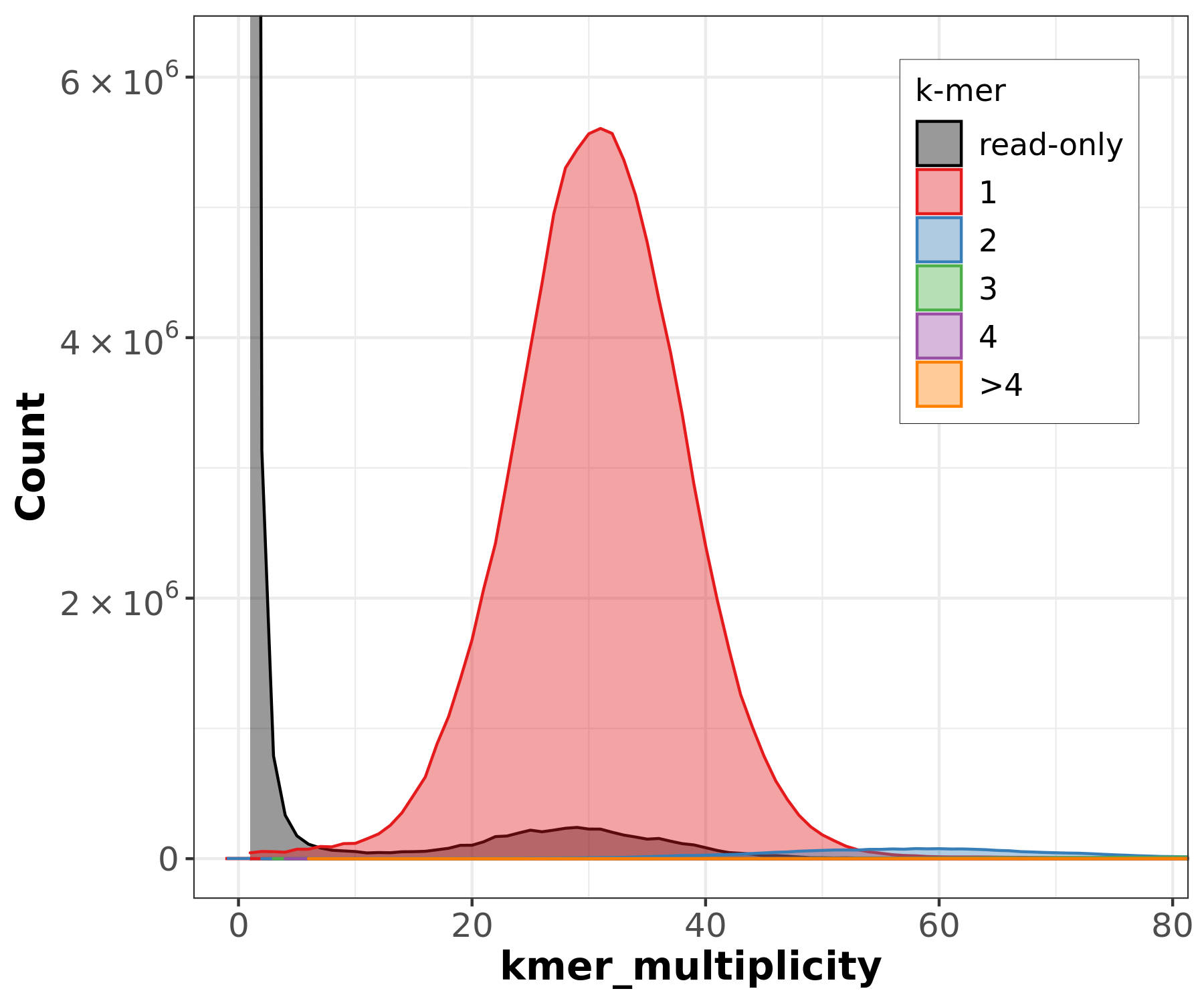
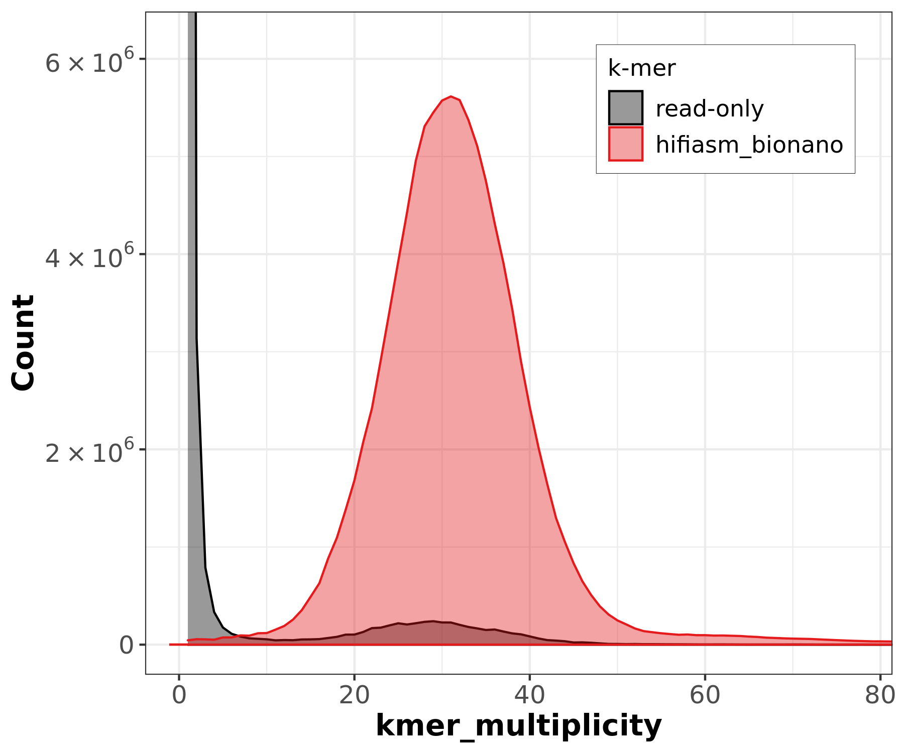
Assembly graph visualization using Bandage
Bandage is a tool for visualizing assembly graphs, which represent the connections between contigs or scaffolds in a genome assembly. By visualizing the graph structure, you can identify complex regions, repetitive elements, and potential misassemblies that may affect the genome reconstruction.
To visualize the assembly graph using Bandage:
- Open a web browser and navigate to desktop.negishi.rcac.purdue.edu.
- Log in with your Purdue Career Account username and password, but append “,push” to your password.
- Launch the terminal and run the following command:
- In the Bandage interface, navigate to your assembly folder and load
your assembly graph in GFA format (e.g.,
../02_pacbio-hifi/hifiasm_default/At_hifiasm_default.asm.bp.p_ctg.gfafor hifiasm, or../03_ont-assembly/flye_ont/assembly_graph.gfafor Flye). - Explore the graph structure, identify complex regions, and visualize connections between contigs or scaffolds.
Bandage input format
Bandage requires assembly graph files
(.gfa format), not FASTA files. HiFiasm outputs
.gfa files directly, while Flye produces
assembly_graph.gfa in its output directory.
Unified Assembly Comparison
After running all evaluation tools, compile your results into a summary table to compare assemblies side by side:
| Metric | HiFiasm (HiFi) | Flye (HiFi) | Flye (ONT) | HiFiasm (ONT) | Hybrid (Flye) | HiFiasm + Bionano | Flye + Bionano |
|---|---|---|---|---|---|---|---|
| # Contigs | 146 | 83 | 50 | 105 | 333 | 153 | 42 |
| Total size (Mb) | 135.75 | 133.68 | 128.74 | 127.42 | 121.11 | 143.79 | 128.97 |
| N50 (Mb) | 7.98 | 5.97 | 11.82 | 11.34 | 4.06 | 14.05 | 15.52 |
| L50 | 7 | 8 | 5 | 6 | 9 | 5 | 4 |
| BUSCO Complete (%) | 97.08 | 99.93 | 100.00 | 99.65 | 99.91 | 97.06 | 100.00 |
| BUSCO Single (%) | 95.97 | 98.89 | 98.93 | 98.61 | 98.50 | 95.97 | 98.93 |
| BUSCO Duplicated (%) | 1.11 | 1.04 | 1.07 | 1.04 | 1.41 | 1.09 | 1.07 |
| Genome fraction (%) | 86.68 | 90.47 | 99.43 | 95.58 | 90.76 | 86.71 | 99.41 |
| Misassemblies | 824 | 484 | 183 | 59 | 480 | 836 | 198 |
| Merqury QV | — | — | — | — | — | 62.91 | — |
| K-mer completeness (%) | — | — | — | — | — | 95.73 | — |
Interpreting your results
When comparing assemblies, consider these questions:
- Which assembly has the highest N50 and lowest number of contigs?
- Which assembly has the best BUSCO completeness?
- How do the Merqury QV scores compare? (Higher QV = fewer base-level errors)
- Did Bionano scaffolding improve contiguity (N50) compared to the unscaffolded assemblies?
- Is the total assembly size close to the expected genome size (~135 Mb for A. thaliana)?
Fill in the table above with your actual results and discuss which assembly strategy produced the best outcome for this dataset.
- QUAST evaluates assembly contiguity and quality metrics.
- Compleasm assesses gene-space completeness in genome assemblies.
- Merqury provides reference-free evaluation based on k-mer analysis.
- Bandage visualizes assembly graphs for structural assessment.