Gene set enrichment analysis
Last updated on 2026-06-16 | Edit this page
Overview
Questions
- What is over-representation analysis and how does it work statistically?
- How do we identify functional pathways and biological themes from DE genes?
- How do we run enrichment analysis for GO, KEGG, and MSigDB gene sets?
- How do we interpret and compare enrichment results across different databases?
- What are the limitations and best practices for enrichment analysis?
Objectives
- Understand the statistical basis of over-representation analysis (ORA).
- Prepare gene lists and background universes from DESeq2 results.
- Run GO enrichment using clusterProfiler and interpret ontology categories.
- Run KEGG pathway enrichment with organism-specific data.
- Perform MSigDB Hallmark enrichment for curated biological signatures.
- Produce and interpret barplots, dotplots, and enrichment maps.
- Compare results across multiple gene set databases.
Introduction
Differential expression analysis identifies individual genes that change between conditions, but interpreting long gene lists is challenging. Gene set enrichment analysis provides biological context by asking: Are genes with specific functions over-represented among the differentially expressed genes?
This episode covers over-representation analysis (ORA), the most common approach for interpreting DE results.
What you need for this episode
- DE results from Episode 05 or 05b
(
DESeq2_results_joined.tsvorDESeq2_kallisto_results.tsv) - RStudio session via Open OnDemand
- Internet connection (for KEGG queries)
Background: Understanding over-representation analysis
What is ORA?
ORA tests whether a predefined gene set contains more DE genes than expected by chance. It answers the question: If I randomly selected the same number of genes from my background, how often would I see this many genes from pathway X?
The statistical test
ORA uses the hypergeometric test (equivalent to Fisher’s exact test), which calculates the probability of observing k or more genes from a pathway given:
- N: Total genes in the background (universe)
- K: Genes in the pathway of interest
- n: Total DE genes in your list
- k: DE genes that are in the pathway
                    Pathway genes    Non-pathway genes
DE genes                 k              n - k
Non-DE genes K - k N - K - n + kThe hypergeometric distribution
The p-value represents the probability of drawing k or more pathway genes when randomly selecting n genes from a population of N genes containing K pathway members:
\[P(X \geq k) = \sum_{i=k}^{\min(K,n)} \frac{\binom{K}{i}\binom{N-K}{n-i}}{\binom{N}{n}}\]
This is a one-tailed test asking if the pathway is over-represented (enriched) in your gene list.
Multiple testing correction
With thousands of gene sets tested, many false positives would occur by chance. We apply false discovery rate (FDR) correction using the Benjamini-Hochberg method:
- Rank all p-values from smallest to largest.
- Calculate adjusted p-value: \(p_{adj} = p \times \frac{n}{rank}\)
- Filter results by adjusted p-value threshold (typically 0.05).
Why the universe matters
The background universe should include all genes that could have been detected as DE in your experiment, typically all genes tested by DESeq2.
Common mistakes: - Using the whole genome (inflates significance). - Using only expressed genes (may miss relevant pathways). - Using a different species’ gene list.
The universe defines what “expected by chance” means. An inappropriate universe leads to misleading results.
Gene set databases
Different databases capture different aspects of biology:
| Database | Description | Best for |
|---|---|---|
| GO BP | Biological Process ontology | Functional processes |
| GO MF | Molecular Function ontology | Protein activities |
| GO CC | Cellular Component ontology | Subcellular localization |
| KEGG | Curated pathways | Metabolic/signaling pathways |
| Reactome | Detailed pathway reactions | Mechanistic understanding |
| MSigDB Hallmark | 50 curated signatures | High-level biological states |
| MSigDB C2 | Curated gene sets | Canonical pathways |
Which database should I use?
There’s no single “best” database. Consider:
- GO: Comprehensive but redundant; many overlapping terms.
- KEGG: Well-curated pathways; limited coverage; requires Entrez IDs.
- Hallmark: Reduced redundancy; easier to interpret; may miss specific pathways.
Best practice: Run multiple databases and look for convergent signals across them.
Step 1: Load DE results and prepare gene lists
Start your RStudio session via Open OnDemand as described in Episode 05, then load the required packages:
Load packages:
R
library(DESeq2)
library(clusterProfiler)
library(org.Mm.eg.db)
library(msigdbr)
library(enrichplot)
library(dplyr)
library(ggplot2)
library(readr)
# Construct the path dynamically
work_dir <- file.path("/scratch/negishi", Sys.getenv("USER"), "rnaseq-workshop")
setwd(work_dir)
Load DESeq2 results from Episode 05:
R
res <- read_tsv("results/deseq2/DESeq2_results_joined.tsv", show_col_types = FALSE)
head(res)
Output:
# A tibble: 6 × 20
  baseMean log2FoldChange  lfcSE        pvalue         padj ensembl_gene_id_version WT_Bcell_mock_rep1 WT_Bcell_mock_rep2 WT_Bcell_mock_rep3 WT_Bcell_mock_rep4
     <dbl>          <dbl>  <dbl>         <dbl>        <dbl> <chr>                                <dbl>              <dbl>              <dbl>              <dbl>
1     259.         -0.703 0.123  0.00000000431 0.0000000268 ENSMUSG00000033845.14                 195.               212.               202.               174.
2     142.          0.244 0.192  0.177         0.256        ENSMUSG00000025903.15                 157.               141.               167.               160.
3     305.         -0.218 0.121  0.0652        0.111        ENSMUSG00000033813.16                 293.               269.               321.               242.
4     241.          0.224 0.129  0.0741        0.123        ENSMUSG00000033793.13                 279.               250.               291.               224.
5     773.          0.231 0.0952 0.0140        0.0286       ENSMUSG00000025907.15                 831.               760.               887.               865.
6     556.          0.126 0.0892 0.152         0.226        ENSMUSG00000051285.18                 608.               616.               560.               540.
# ℹ 10 more variables: WT_Bcell_IR_rep1 <dbl>, WT_Bcell_IR_rep2 <dbl>, WT_Bcell_IR_rep3 <dbl>, WT_Bcell_IR_rep4 <dbl>, ensembl_gene_id <chr>,
#   external_gene_name <chr>, gene_biotype <chr>, description <chr>, label <chr>, sig <chr>
Define the gene lists:
R
# Universe: all genes tested
universe <- res$ensembl_gene_id_version

# Significant genes: padj < 0.05 and |log2FC| > log2(1.5)
log2fc_cut <- log2(1.5)
sig_genes <- res %>%
    filter(padj < 0.05, abs(log2FoldChange) > log2fc_cut) %>%
    pull(ensembl_gene_id_version)

length(universe)
length(sig_genes)
[1] 11330
[1] 3597Choosing significance thresholds
The threshold for “significant” genes affects enrichment results:
- Stringent (padj < 0.01, |LFC| > 1): Fewer genes, clearer signals, may miss subtle effects.
- Lenient (padj < 0.1, no LFC cutoff): More genes, noisier results, higher sensitivity.
There’s no universally correct threshold. Consider your experimental question and validate key findings.
Convert gene IDs
Most enrichment tools require Entrez IDs. Our data uses Ensembl IDs with version numbers, so we need to convert:
R
# Remove version suffix for mapping
universe_clean <- gsub("\\.\\d+$", "", universe)
sig_clean <- gsub("\\.\\d+$", "", sig_genes)

# Map Ensembl to Entrez
id_map <- bitr(
    universe_clean,
    fromType = "ENSEMBL",
    toType = "ENTREZID",
    OrgDb = org.Mm.eg.db
)

head(id_map)
             ENSEMBL ENTREZID
1 ENSMUSG00000033845    27395
2 ENSMUSG00000025903    18777
3 ENSMUSG00000033813    21399
4 ENSMUSG00000033793   108664
5 ENSMUSG00000025907    12421
6 ENSMUSG00000051285 319263Gene ID conversion challenges
Not all genes map successfully:
- Some Ensembl IDs lack Entrez equivalents.
- ID mapping databases may be outdated.
- Multi-mapping (one Ensembl → multiple Entrez) can occur.
bitr() drops unmapped genes silently. Check how many
genes were lost:
R
message(sprintf("Mapped %d of %d genes (%.1f%%)",
    nrow(id_map), length(universe_clean),
    100 * nrow(id_map) / length(universe_clean)))
Output:
Mapped 11358 of 11330 genes (100.2%)Create final gene lists with Entrez IDs:
R
# Universe with Entrez IDs
universe_entrez <- id_map$ENTREZID

# Significant genes with Entrez IDs
sig_entrez <- id_map %>%
    filter(ENSEMBL %in% sig_clean) %>%
    pull(ENTREZID)

length(sig_entrez)
Output:
[1] 3608Exercise: Prepare up-regulated and down-regulated gene lists
Create separate gene lists for: 1. Up-regulated genes (log2FC > 0 and padj < 0.05) 2. Down-regulated genes (log2FC < 0 and padj < 0.05)
Why might analyzing these separately be informative?
R
# Up-regulated genes
up_genes <- res %>%
    filter(padj < 0.05, log2FoldChange > log2fc_cut) %>%
    pull(ensembl_gene_id_version)
up_clean <- gsub("\\.\\d+$", "", up_genes)
up_entrez <- id_map %>%
    filter(ENSEMBL %in% up_clean) %>%
    pull(ENTREZID)

# Down-regulated genes
down_genes <- res %>%
    filter(padj < 0.05, log2FoldChange < -log2fc_cut) %>%
    pull(ensembl_gene_id_version)
down_clean <- gsub("\\.\\d+$", "", down_genes)
down_entrez <- id_map %>%
    filter(ENSEMBL %in% down_clean) %>%
    pull(ENTREZID)
Check number of genes:
R
length(up_entrez)
[1] 1810R
length(down_entrez)
[1] 1798Analyzing up and down separately can reveal: - Different biological processes activated vs. suppressed. - Clearer signals when combining masks opposing effects. - Direction-specific pathway involvement.
Step 2: GO enrichment analysis
Run GO Biological Process enrichment
R
ego_bp <- enrichGO(
    gene = sig_entrez,
    universe = universe_entrez,
    OrgDb = org.Mm.eg.db,
    ont = "BP",
    pAdjustMethod = "BH",
    pvalueCutoff = 0.05,
    qvalueCutoff = 0.1,
    readable = TRUE
)

head(ego_bp, 10)
Output (columns truncated for brevity):
                   ID                                    Description GeneRatio   BgRatio RichFactor FoldEnrichment   zScore       pvalue    p.adjust      qvalue
GO:0002683 GO:0002683   negative regulation of immune system process  174/3494 405/10989  0.4296296       1.351231 4.917337 1.003906e-06 0.005247415 0.004941330
GO:0042100 GO:0042100                           B cell proliferation   44/3494  77/10989  0.5714286       1.797203 4.792888 3.631972e-06 0.009166217 0.008631545
GO:0032943 GO:0032943                 mononuclear cell proliferation  119/3494 266/10989  0.4473684       1.407021 4.588117 5.260886e-06 0.009166217 0.008631545
GO:0051250 GO:0051250   negative regulation of lymphocyte activation   65/3494 130/10989  0.5000000       1.572553 4.483605 1.087013e-05 0.012782384 0.012036778
GO:0046651 GO:0046651                       lymphocyte proliferation  115/3494 260/10989  0.4423077       1.391105 4.357475 1.428670e-05 0.012782384 0.012036778
GO:0002698 GO:0002698 negative regulation of immune effector process   51/3494  97/10989  0.5257732       1.653612 4.414558 1.636446e-05 0.012782384 0.012036778
GO:0042254 GO:0042254                            ribosome biogenesis  131/3494 304/10989  0.4309211       1.355292 4.289141 1.808829e-05 0.012782384 0.012036778
GO:0042113 GO:0042113                              B cell activation  107/3494 241/10989  0.4439834       1.396375 4.248012 2.305909e-05 0.012782384 0.012036778
GO:0006364 GO:0006364                                rRNA processing   95/3494 210/10989  0.4523810       1.422786 4.223534 2.665078e-05 0.012782384 0.012036778
GO:0002694 GO:0002694 regulation of leukocyte activation 189/3494 466/10989 0.4055794 1.275590 4.150705 2.844730e-05 0.012782384 0.012036778Understanding enrichGO output
Key columns in the results:
- ID: GO term identifier (e.g., GO:0006915)
- Description: Human-readable term name
- GeneRatio: DE genes in term / total DE genes with annotation
- BgRatio: Term genes in universe / total annotated genes in universe
- pvalue: Raw hypergeometric p-value
- p.adjust: BH-corrected p-value
- qvalue: Alternative FDR estimate
- geneID: List of DE genes in this term
- Count: Number of DE genes in this term
Visualize GO results
Dotplot showing top enriched terms:
R
dotplot(ego_bp, showCategory = 20) +
    ggtitle("GO Biological Process enrichment")
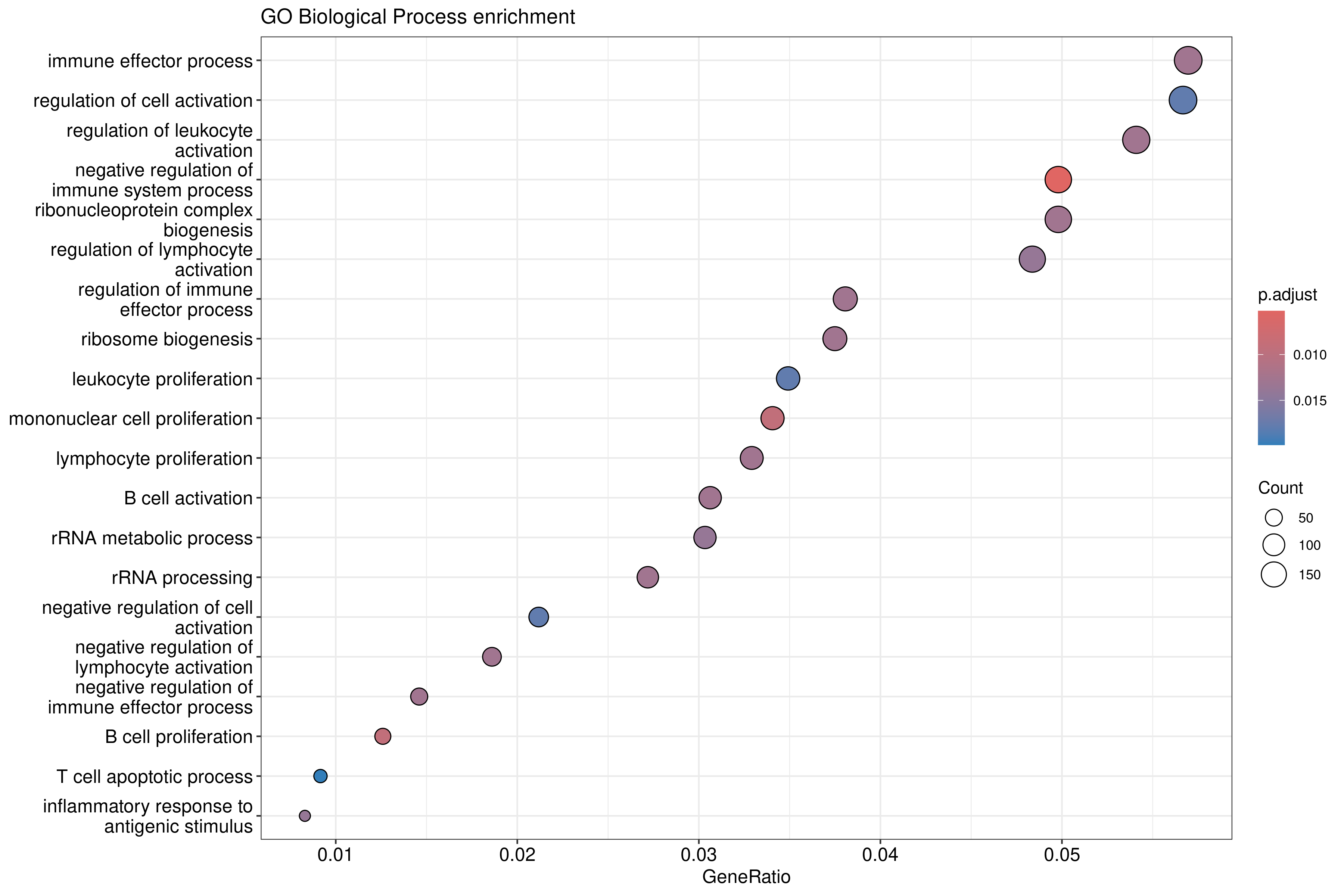
The dotplot shows: - X-axis: Gene ratio (proportion of DE genes in the term) - Y-axis: GO term description - Color: Adjusted p-value - Size: Number of genes
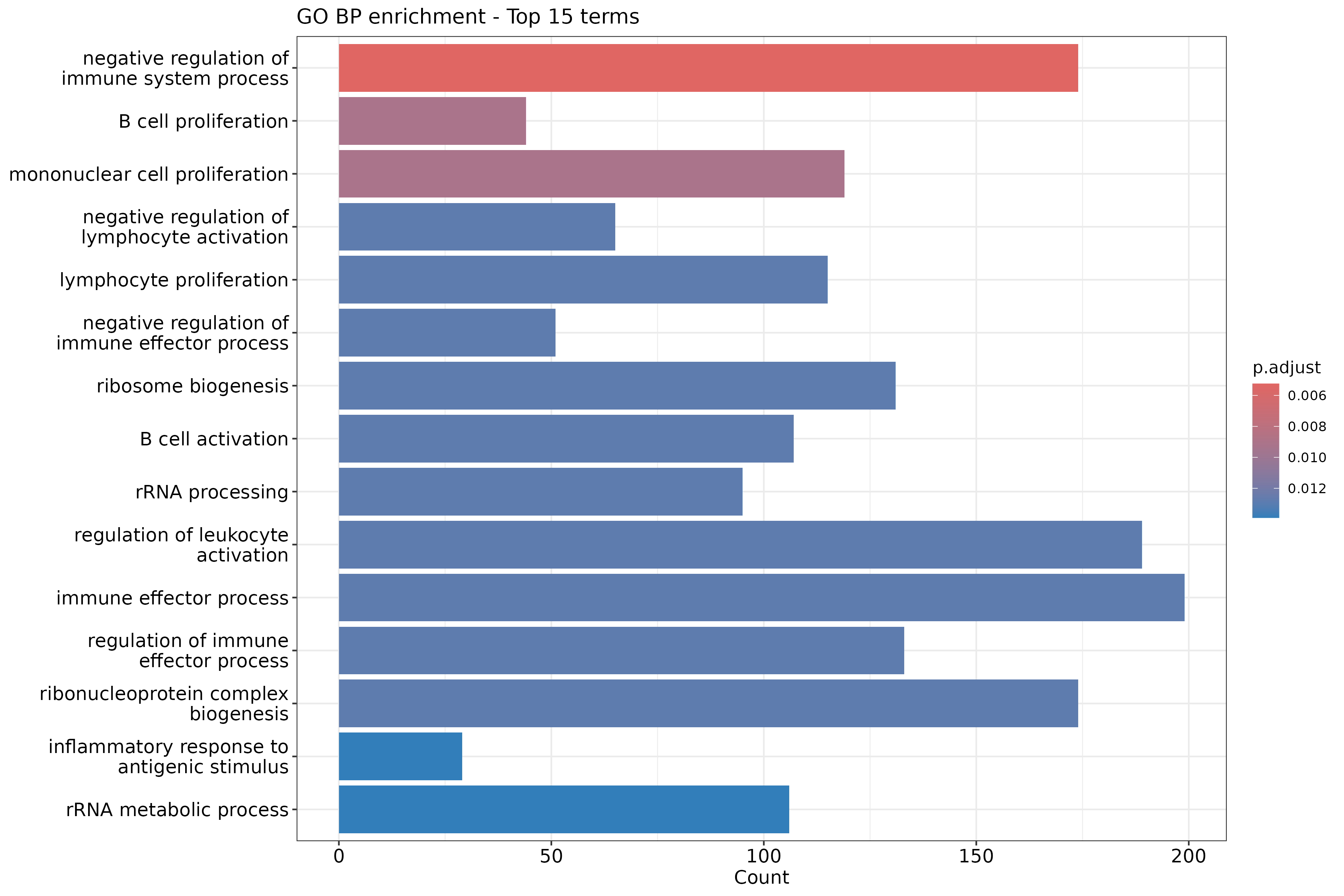
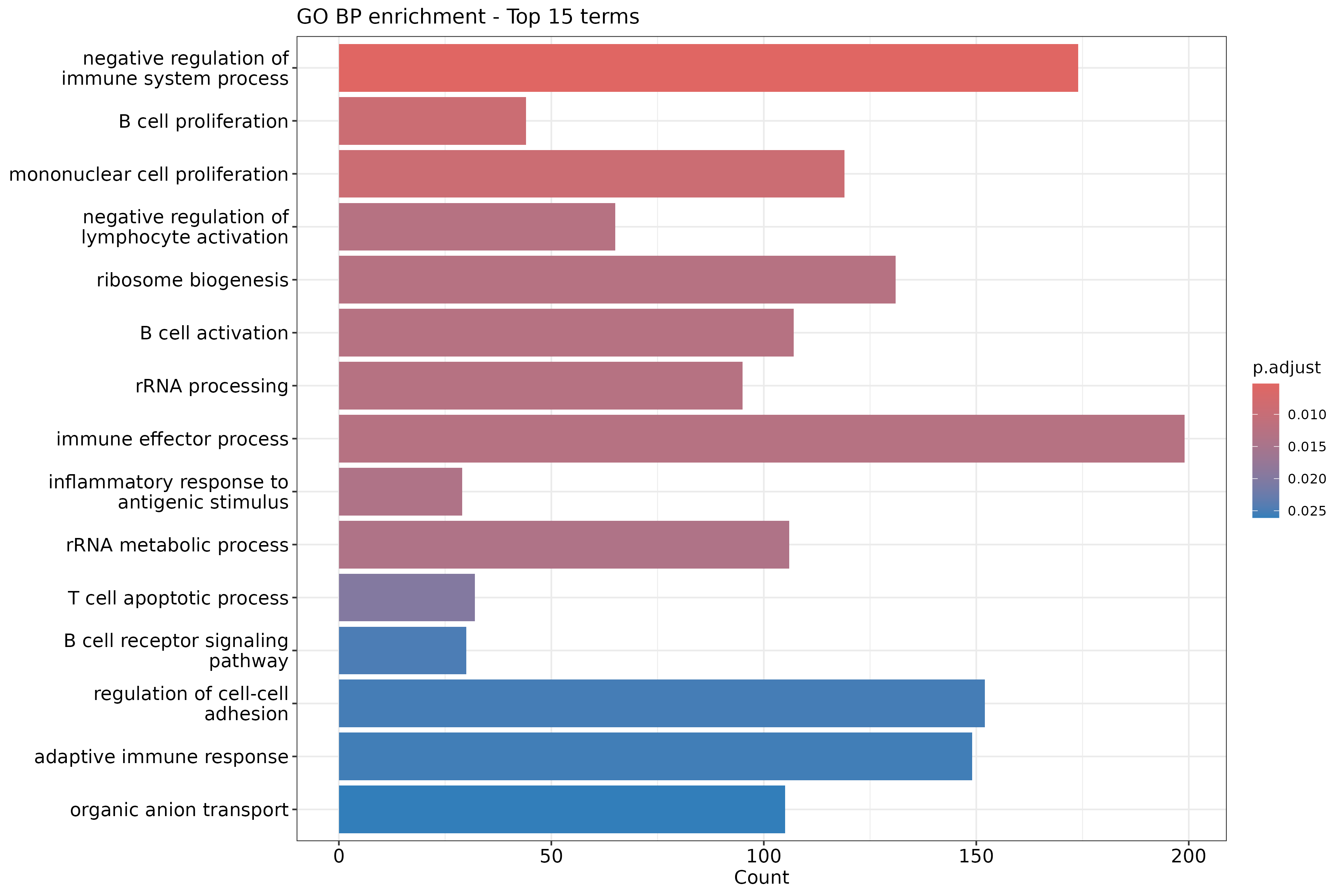
Barplot alternative:
R
barplot(ego_bp, showCategory = 15) +
    ggtitle("GO BP enrichment - Top 15 terms")
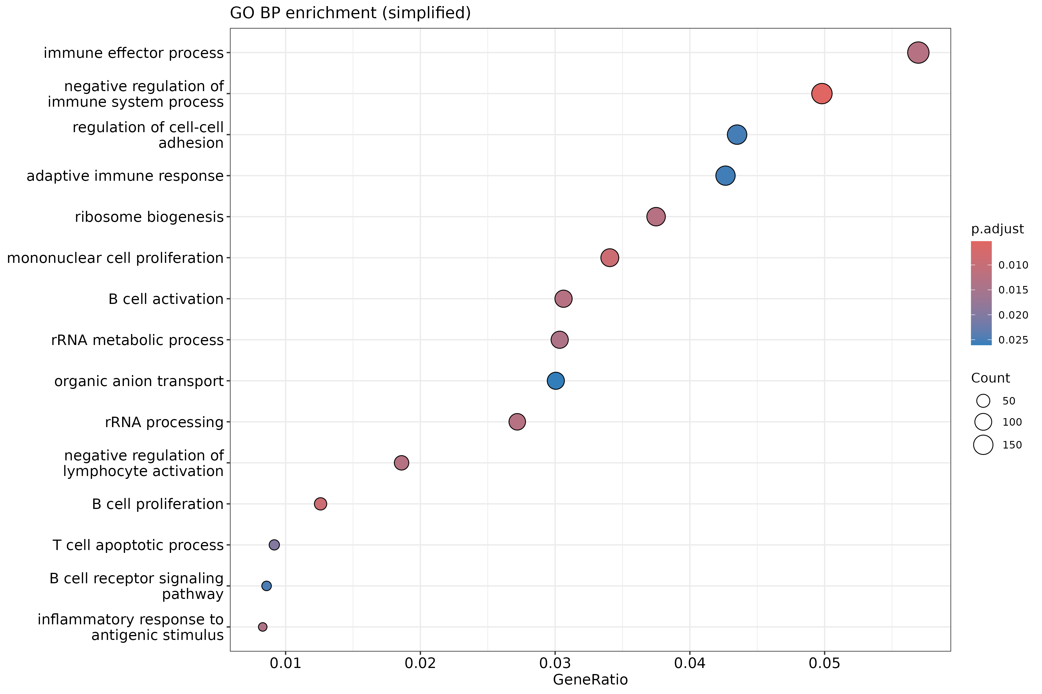
Reduce GO redundancy
GO terms are hierarchical and often redundant. Use
simplify() to remove similar terms:
R
ego_bp_simple <- simplify(
    ego_bp,
    cutoff = 0.7,
    by = "p.adjust",
    select_fun = min
)

dotplot(ego_bp_simple, showCategory = 15) +
    ggtitle("GO BP enrichment (simplified)")
Why simplify GO results?
The GO hierarchy means related terms often appear together: - “regulation of cell death” and “positive regulation of cell death” - “response to stimulus” and “response to external stimulus”
simplify() removes redundant terms based on semantic
similarity, making results easier to interpret. The cutoff
parameter (0-1) controls how aggressively terms are merged.
Enrichment map visualization
For many significant terms, an enrichment map shows relationships:
R
ego_bp_em <- pairwise_termsim(ego_bp_simple)
emapplot(ego_bp_em, showCategory = 30) +
    ggtitle("GO BP enrichment map")
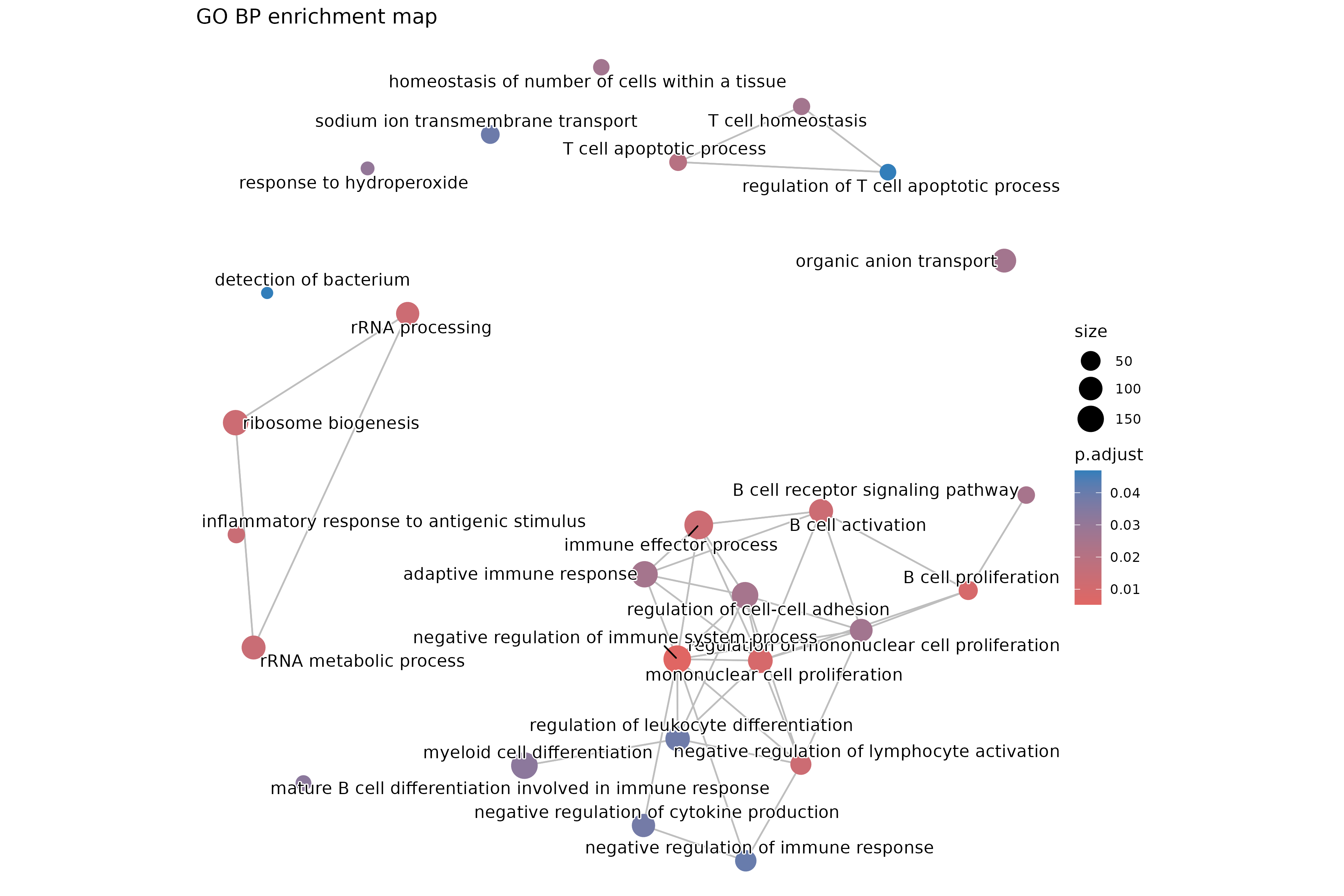
The enrichment map clusters similar terms together, revealing functional themes.
Exercise: Compare GO ontologies
Run enrichment for GO Molecular Function (MF) and Cellular Component (CC):
R
ego_mf <- enrichGO(gene = sig_entrez, universe = universe_entrez,
                   OrgDb = org.Mm.eg.db, ont = "MF", readable = TRUE)
ego_cc <- enrichGO(gene = sig_entrez, universe = universe_entrez,
                   OrgDb = org.Mm.eg.db, ont = "CC", readable = TRUE)
- How do the top terms differ between BP, MF, and CC?
- Are there consistent themes across ontologies?
- Which ontology provides the most interpretable results for your experiment?
Example interpretation:
- BP terms describe processes (e.g., “cell cycle”, “RNA processing”).
- MF terms describe molecular activities (e.g., “RNA binding”, “kinase activity”).
- CC terms describe locations (e.g., “nucleus”, “mitochondrion”).
Consistent themes across ontologies strengthen biological interpretation. For example, if BP shows “translation” enrichment, MF might show “ribosome binding”, and CC might show “ribosome” or “cytoplasm”.
Step 3: KEGG pathway enrichment
KEGG provides curated pathway maps connecting genes to biological systems.
R
ekegg <- enrichKEGG(
    gene = sig_entrez,
    universe = universe_entrez,
    organism = "mmu",  # Mouse
    pAdjustMethod = "BH",
    pvalueCutoff = 0.05
)

head(ekegg)
Output (geneID column not shown for brevity):
                                    category                         subcategory       ID                              Description GeneRatio BgRatio RichFactor
mmu04115                   Cellular Processes               Cell growth and death mmu04115                    p53 signaling pathway   41/1686 64/5208  0.6406250
mmu05322                       Human Diseases                      Immune disease mmu05322             Systemic lupus erythematosus   46/1686 87/5208  0.5287356
mmu04977                   Organismal Systems                    Digestive system mmu04977         Vitamin digestion and absorption   12/1686 15/5208  0.8000000
mmu04514 Environmental Information Processing Signaling molecules and interaction mmu04514 Cell adhesion molecule (CAM) interaction   43/1686 85/5208  0.5058824
mmu05150                       Human Diseases       Infectious disease: bacterial mmu05150          Staphylococcus aureus infection   19/1686 30/5208  0.6333333
mmu04981                                 <NA>                                <NA> mmu04981          Folate transport and metabolism   13/1686 18/5208  0.7222222
         FoldEnrichment   zScore       pvalue     p.adjust       qvalue
mmu04115       1.978870 5.451204 1.688415e-07 5.605537e-05 5.491791e-05
mmu05322       1.633247 4.120819 5.329885e-05 8.847610e-03 8.668077e-03
mmu04977       2.471174 3.947558 2.042589e-04 2.260466e-02 2.214597e-02
mmu04514       1.562654 3.618403 3.393132e-04 2.816300e-02 2.759152e-02
mmu05150       1.956346 3.634316 4.705801e-04 3.124652e-02 3.061248e-02
mmu04981       2.230921 3.619185 6.082405e-04 3.365597e-02 3.297304e-02
         Count
mmu04115    41
mmu05322    46
mmu04977    12
mmu04514    43
mmu05150    19
mmu04981 13KEGG organism codes
Common organism codes: - "hsa": Human -
"mmu": Mouse - "rno": Rat -
"dme": Drosophila - "sce": Yeast -
"ath": Arabidopsis
Find your organism:
search_kegg_organism("species name")
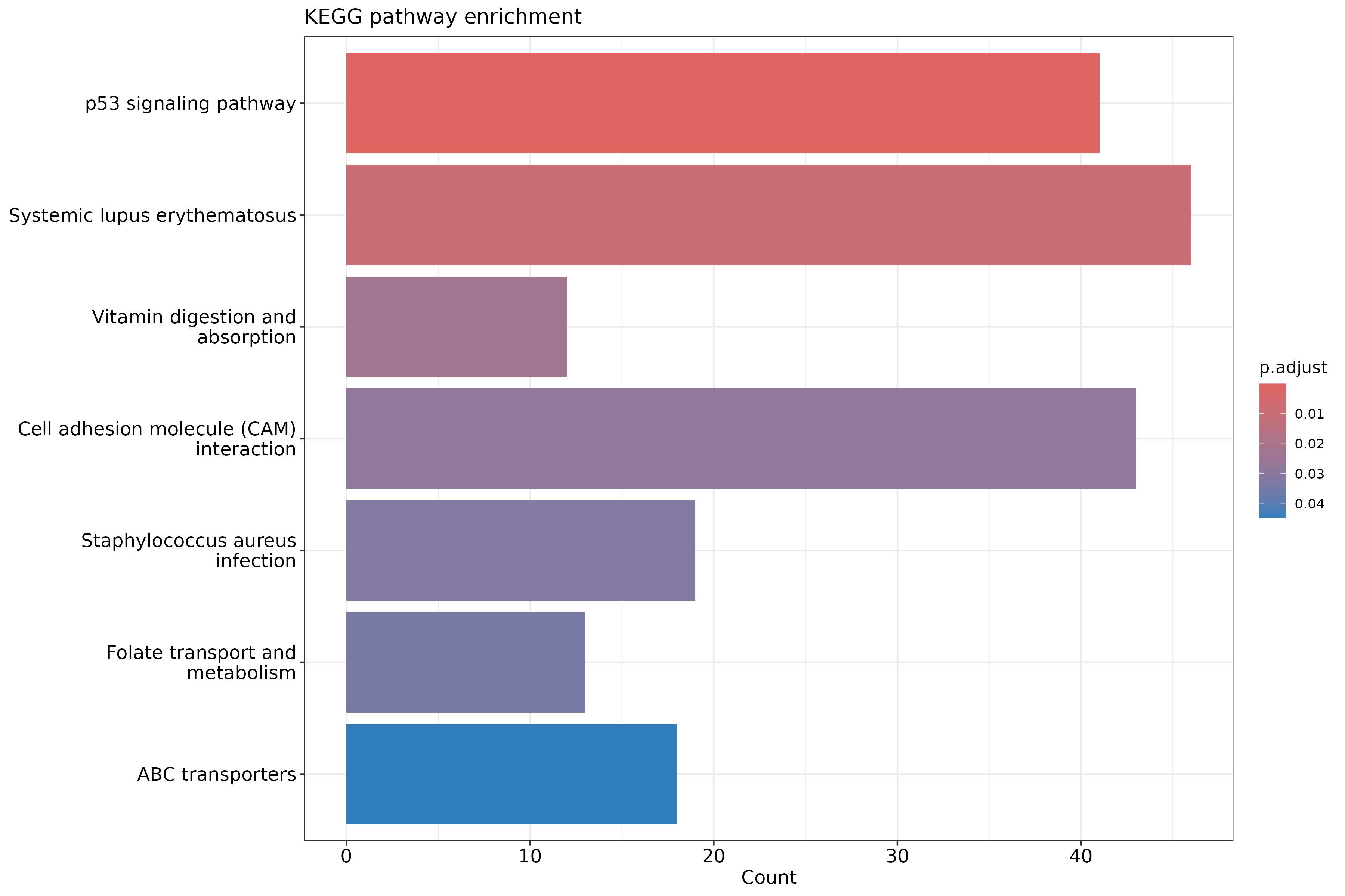
Visualize KEGG results:
R
barplot(ekegg, showCategory = 15) +
    ggtitle("KEGG pathway enrichment")
KEGG limitations
Be aware of KEGG-specific issues:
- ID coverage: KEGG uses its own gene IDs; some Entrez IDs may not map.
- Update frequency: KEGG pathways are updated periodically; results may vary.
- License: KEGG has usage restrictions for commercial applications.
- Incomplete mapping: Some genes lack pathway assignments.
Check dropped genes:
R
message(sprintf("KEGG analysis used %d of %d input genes",
    length(ekegg@gene), length(sig_entrez)))
Output:
KEGG analysis used 3607 of 3608 input genesStep 4: MSigDB Hallmark enrichment
MSigDB Hallmark gene sets are 50 curated signatures representing well-defined biological states and processes.
Load Hallmark gene sets
R
hallmark <- msigdbr(species = "Mus musculus", category = "H")
head(hallmark)
Output:
# A tibble: 6 × 26
  gene_symbol ncbi_gene ensembl_gene       db_gene_symbol db_ncbi_gene db_ensembl_gene source_gene gs_id gs_name  gs_collection gs_subcollection gs_collection_name
  <chr>       <chr>     <chr>              <chr>          <chr>        <chr>           <chr>       <chr> <chr>    <chr>         <chr>            <chr>
1 Abca1       11303     ENSMUSG00000015243 ABCA1          19           ENSG00000165029 ABCA1       M5905 HALLMAR… H             ""               Hallmark
2 Abcb8       74610     ENSMUSG00000028973 ABCB8          11194        ENSG00000197150 ABCB8       M5905 HALLMAR… H             ""               Hallmark
3 Acaa2       52538     ENSMUSG00000036880 ACAA2          10449        ENSG00000167315 ACAA2       M5905 HALLMAR… H             ""               Hallmark
4 Acadl       11363     ENSMUSG00000026003 ACADL          33           ENSG00000115361 ACADL       M5905 HALLMAR… H             ""               Hallmark
5 Acadm       11364     ENSMUSG00000062908 ACADM          34           ENSG00000117054 ACADM       M5905 HALLMAR… H             ""               Hallmark
6 Acads       11409     ENSMUSG00000029545 ACADS          35           ENSG00000122971 ACADS       M5905 HALLMAR… H             ""               Hallmark
# ℹ 14 more variables: gs_description <chr>, gs_source_species <chr>, gs_pmid <chr>, gs_geoid <chr>, gs_exact_source <chr>, gs_url <chr>, db_version <chr>,
#   db_target_species <chr>, ortholog_taxon_id <int>, ortholog_sources <chr>, num_ortholog_sources <dbl>, entrez_gene <chr>, gs_cat <chr>, gs_subcat <chr>
Prepare gene set list:
R
hallmark_list <- hallmark %>%
    dplyr::select(gs_name, entrez_gene) %>%
    dplyr::rename(term = gs_name, gene = entrez_gene)
Run Hallmark enrichment
R
ehall <- enricher(
    gene = sig_entrez,
    universe = universe_entrez,
    TERM2GENE = hallmark_list,
    pAdjustMethod = "BH",
    pvalueCutoff = 0.05
)

head(ehall)
Output (columns truncated for brevity):
                                             ID             Description GeneRatio  BgRatio RichFactor FoldEnrichment   zScore       pvalue     p.adjust
HALLMARK_MYC_TARGETS_V2 HALLMARK_MYC_TARGETS_V2 HALLMARK_MYC_TARGETS_V2   40/1134  57/3216  0.7017544       1.990161 5.565765 6.573980e-08 3.286990e-06
HALLMARK_P53_PATHWAY       HALLMARK_P53_PATHWAY    HALLMARK_P53_PATHWAY   86/1134 164/3216  0.5243902       1.487160 4.725607 2.814573e-06 7.036433e-05
Visualize:
R
dotplot(ehall, showCategory = 20) +
    ggtitle("MSigDB Hallmark enrichment")
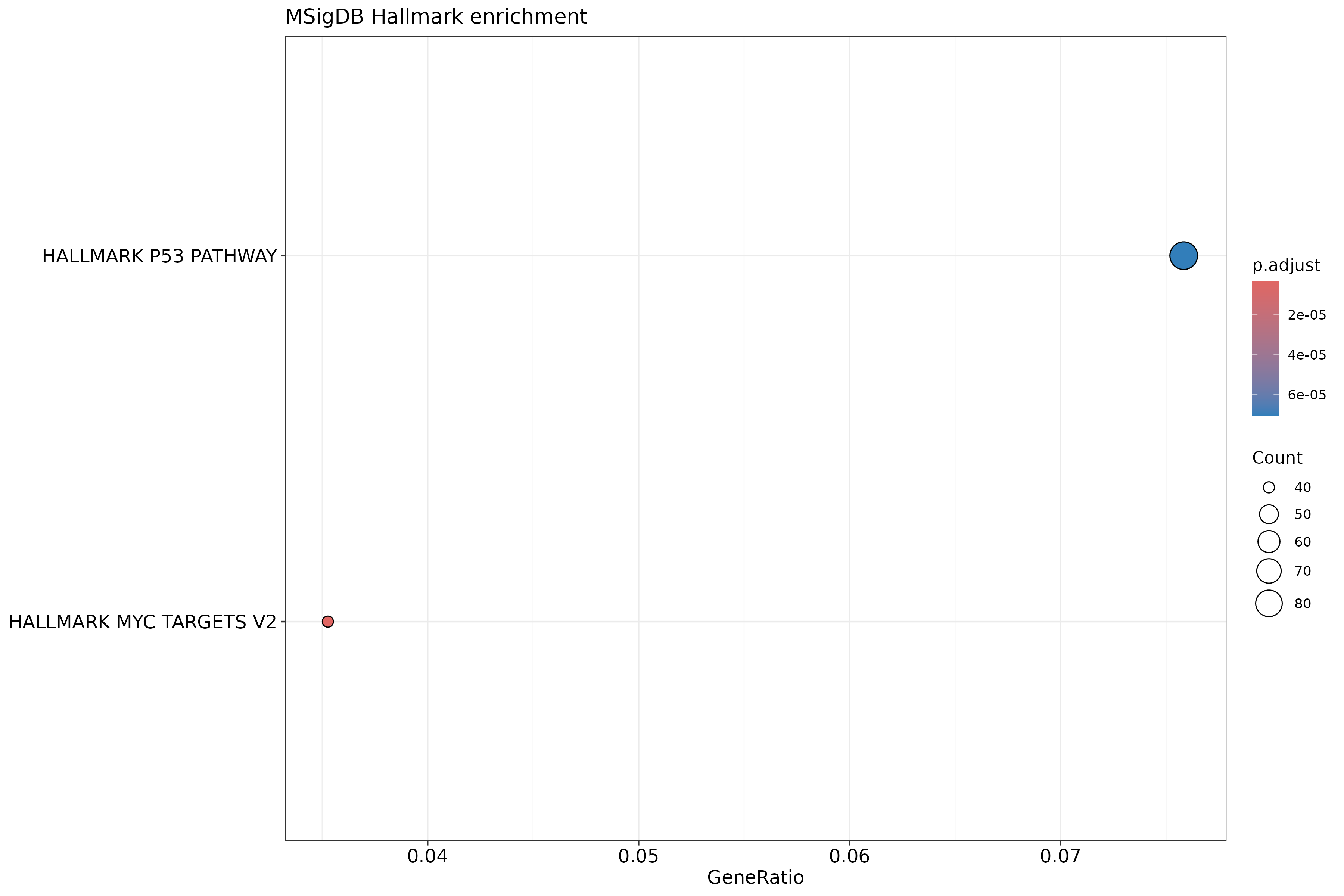
Why use Hallmark gene sets?
Advantages of Hallmark over GO/KEGG:
- Reduced redundancy: Each signature is distinct and non-overlapping.
- Expert curation: Refined from multiple sources to represent coherent biology.
- Interpretability: 50 sets is manageable for detailed examination.
- Reproducibility: Well-documented and stable definitions.
Common Hallmark sets include: - HALLMARK_INFLAMMATORY_RESPONSE - HALLMARK_P53_PATHWAY - HALLMARK_OXIDATIVE_PHOSPHORYLATION - HALLMARK_MYC_TARGETS_V1
Step 5: Compare results across databases
Create a summary of top enriched terms from each database:
R
# Extract top 10 from each
top_go <- head(ego_bp_simple@result, 10) %>%
    mutate(Database = "GO BP") %>%
    dplyr::select(Database, Description, p.adjust, Count)

top_kegg <- head(ekegg@result, 10) %>%
    mutate(Database = "KEGG") %>%
    dplyr::select(Database, Description, p.adjust, Count)

top_hall <- head(ehall@result, 10) %>%
    mutate(Database = "Hallmark") %>%
    dplyr::select(Database, ID, p.adjust, Count) %>%
    dplyr::rename(Description = ID)

# Combine
comparison <- bind_rows(top_go, top_kegg, top_hall)
comparison
Output:
                                 Database                                  Description     p.adjust Count
GO:0002683                          GO BP negative regulation of immune system process 5.247415e-03   174
GO:0042100                          GO BP                         B cell proliferation 9.166217e-03    44
GO:0032943                          GO BP               mononuclear cell proliferation 9.166217e-03   119
GO:0051250                          GO BP negative regulation of lymphocyte activation 1.278238e-02    65
GO:0042254                          GO BP                          ribosome biogenesis 1.278238e-02   131
GO:0042113                          GO BP                            B cell activation 1.278238e-02   107
GO:0006364                          GO BP                              rRNA processing 1.278238e-02    95
GO:0002252                          GO BP                      immune effector process 1.278238e-02   199
GO:0002437                          GO BP  inflammatory response to antigenic stimulus 1.390022e-02    29
GO:0016072                          GO BP                       rRNA metabolic process 1.390022e-02   106
mmu04115                             KEGG                        p53 signaling pathway 5.605537e-05    41
mmu05322                             KEGG                 Systemic lupus erythematosus 8.847610e-03    46
mmu04977                             KEGG             Vitamin digestion and absorption 2.260466e-02    12
mmu04514                             KEGG     Cell adhesion molecule (CAM) interaction 2.816300e-02    43
mmu05150                             KEGG              Staphylococcus aureus infection 3.124652e-02    19
mmu04981                             KEGG              Folate transport and metabolism 3.365597e-02    13
mmu02010                             KEGG                             ABC transporters 4.462944e-02    18
mmu03008                             KEGG            Ribosome biogenesis in eukaryotes 8.758267e-02    35
mmu05202                             KEGG      Transcriptional misregulation in cancer 9.020508e-02    60
mmu04068                             KEGG                       FoxO signaling pathway 1.135249e-01    48
HALLMARK_MYC_TARGETS_V2          Hallmark                      HALLMARK_MYC_TARGETS_V2 3.286990e-06    40
HALLMARK_P53_PATHWAY             Hallmark                         HALLMARK_P53_PATHWAY 7.036433e-05    86
HALLMARK_XENOBIOTIC_METABOLISM   Hallmark               HALLMARK_XENOBIOTIC_METABOLISM 1.034831e-01    57
HALLMARK_HEME_METABOLISM         Hallmark                     HALLMARK_HEME_METABOLISM 1.034831e-01    72
HALLMARK_IL2_STAT5_SIGNALING     Hallmark                 HALLMARK_IL2_STAT5_SIGNALING 1.611589e-01    69
HALLMARK_ALLOGRAFT_REJECTION     Hallmark                 HALLMARK_ALLOGRAFT_REJECTION 1.611589e-01    70
HALLMARK_MYC_TARGETS_V1          Hallmark                      HALLMARK_MYC_TARGETS_V1 1.757524e-01    84
HALLMARK_TNFA_SIGNALING_VIA_NFKB Hallmark             HALLMARK_TNFA_SIGNALING_VIA_NFKB 2.021817e-01    67
HALLMARK_ESTROGEN_RESPONSE_EARLY Hallmark             HALLMARK_ESTROGEN_RESPONSE_EARLY 2.021817e-01    56
HALLMARK_APOPTOSIS Hallmark HALLMARK_APOPTOSIS 2.527274e-01 54Exercise: Identify convergent themes
Looking at your GO, KEGG, and Hallmark results:
- Are there biological themes that appear across multiple databases?
- Are there database-specific findings that don’t replicate elsewhere?
- How would you prioritize which findings to investigate further?
Convergent signals to look for:
- If GO shows “cell cycle” terms, KEGG might show “Cell cycle” pathway, and Hallmark might show “HALLMARK_G2M_CHECKPOINT”.
- If GO shows “immune response”, KEGG might show “Cytokine-cytokine receptor interaction”, and Hallmark might show “HALLMARK_INFLAMMATORY_RESPONSE”.
Database-specific findings may indicate: - Pathway coverage differences. - Annotation biases. - Potentially spurious signals (require validation).
Prioritization strategy: 1. Focus on themes appearing in multiple databases. 2. Consider effect size (how many genes, fold enrichment). 3. Assess biological plausibility given experimental design. 4. Validate key findings with independent methods.
Step 5b: Direction-aware enrichment analysis
ORA on all significant genes (up + down combined) can mask biological signals when up-regulated and down-regulated genes have different functions. Analyzing directions separately often reveals clearer patterns.
Prepare direction-specific gene lists
R
# Up-regulated genes
up_genes <- res %>%
    filter(padj < 0.05, log2FoldChange > log2fc_cut) %>%
    pull(ensembl_gene_id_version)
up_clean <- gsub("\\.\\d+$", "", up_genes)
up_entrez <- id_map %>%
    filter(ENSEMBL %in% up_clean) %>%
    pull(ENTREZID)

# Down-regulated genes
down_genes <- res %>%
    filter(padj < 0.05, log2FoldChange < -log2fc_cut) %>%
    pull(ensembl_gene_id_version)
down_clean <- gsub("\\.\\d+$", "", down_genes)
down_entrez <- id_map %>%
    filter(ENSEMBL %in% down_clean) %>%
    pull(ENTREZID)

message(sprintf("Up-regulated: %d genes, Down-regulated: %d genes",
    length(up_entrez), length(down_entrez)))
Up-regulated: 1810 genes, Down-regulated: 1798 genesRun enrichment for each direction
R
# GO enrichment for up-regulated genes
ego_up <- enrichGO(
    gene = up_entrez,
    universe = universe_entrez,
    OrgDb = org.Mm.eg.db,
    ont = "BP",
    readable = TRUE
)

# GO enrichment for down-regulated genes
ego_down <- enrichGO(
    gene = down_entrez,
    universe = universe_entrez,
    OrgDb = org.Mm.eg.db,
    ont = "BP",
    readable = TRUE
)
Compare directions
R
# Combine top results for comparison
up_top <- head(ego_up@result, 10) %>%
    mutate(Direction = "Up-regulated") %>%
    dplyr::select(Direction, Description, p.adjust, Count)

down_top <- head(ego_down@result, 10) %>%
    mutate(Direction = "Down-regulated") %>%
    dplyr::select(Direction, Description, p.adjust, Count)

direction_comparison <- bind_rows(up_top, down_top)
direction_comparison
Output:
                Direction                                                                              Description     p.adjust Count
GO:0002694   Up-regulated                                                       regulation of leukocyte activation 7.705961e-07   127
GO:0002683   Up-regulated                                             negative regulation of immune system process 9.130747e-07   113
GO:0050865   Up-regulated                                                            regulation of cell activation 1.389200e-06   131
GO:0002252   Up-regulated                                                                  immune effector process 1.389200e-06   130
GO:0007264   Up-regulated                                                small GTPase-mediated signal transduction 2.781020e-06    95
GO:0051249   Up-regulated                                                      regulation of lymphocyte activation 4.543747e-06   111
GO:0009617   Up-regulated                                                                    response to bacterium 4.720694e-06   120
GO:0002697   Up-regulated                                                    regulation of immune effector process 1.175944e-05    88
GO:0007186   Up-regulated                                             G protein-coupled receptor signaling pathway 1.175944e-05    97
GO:0030036   Up-regulated                                                          actin cytoskeleton organization 3.108071e-05   123
GO:0022613 Down-regulated                                                     ribonucleoprotein complex biogenesis 2.154137e-27   164
GO:0042254 Down-regulated                                                                      ribosome biogenesis 3.115494e-25   128
GO:0006364 Down-regulated                                                                          rRNA processing 4.368810e-19    92
GO:0016072 Down-regulated                                                                   rRNA metabolic process 6.776964e-19   100
GO:0042273 Down-regulated                                                       ribosomal large subunit biogenesis 1.090959e-08    33
GO:0042274 Down-regulated                                                       ribosomal small subunit biogenesis 4.296891e-08    45
GO:0006399 Down-regulated                                                                   tRNA metabolic process 1.002785e-06    62
GO:0000470 Down-regulated                                                                   maturation of LSU-rRNA 2.496138e-05    17
GO:0009451 Down-regulated                                                                         RNA modification 4.970122e-05    48
GO:0000463 Down-regulated maturation of LSU-rRNA from tricistronic rRNA transcript (SSU-rRNA, 5.8S rRNA, LSU-rRNA) 7.457449e-05 13When to analyze directions separately
Separate analysis is particularly useful when:
- You expect different biological processes to be activated vs. suppressed.
- Combined analysis shows few significant results (opposing signals may cancel out).
- You want to understand mechanism (what’s gained vs. lost).
Separate analysis is less useful when:
- You have very few DE genes in one direction.
- The biological question is about overall pathway disruption.
Step 5c: Gene Set Enrichment Analysis (GSEA)
ORA has a fundamental limitation: it requires an arbitrary cutoff to define “significant” genes. GSEA uses the full ranked gene list without cutoffs.
How GSEA differs from ORA
| Aspect | ORA | GSEA |
|---|---|---|
| Input | List of significant genes | All genes, ranked by fold change |
| Cutoff | Required (padj, LFC) | None |
| Sensitivity | May miss coordinated small changes | Detects subtle but consistent shifts |
| Gene weights | All DE genes treated equally | Magnitude of change matters |
Prepare ranked gene list for GSEA
GSEA requires a named vector of gene scores (typically log2 fold change or a signed significance score):
R
# Create ranked list using signed -log10(pvalue) * sign(LFC)
# This weights by both significance and direction
res_gsea <- res %>%
    filter(!is.na(padj), !is.na(log2FoldChange)) %>%
    mutate(
        ensembl_clean = gsub("\\.\\d+$", "", ensembl_gene_id_version),
        rank_score = -log10(pvalue) * sign(log2FoldChange)
    )

# Map to Entrez IDs
res_gsea <- res_gsea %>%
    inner_join(id_map, by = c("ensembl_clean" = "ENSEMBL"))

# Create named vector (required format for GSEA)
gene_list <- res_gsea$rank_score
names(gene_list) <- res_gsea$ENTREZID

# Sort by rank score (required for GSEA)
gene_list <- sort(gene_list, decreasing = TRUE)
Run GSEA with clusterProfiler
R
# 1. Sort the list in decreasing order (required by clusterProfiler)
gene_list <- sort(gene_list, decreasing = TRUE)
# 2. Remove duplicate Entrez IDs
# (Since we sorted by value, this keeps the instance with the highest absolute value)
gene_list <- gene_list[!duplicated(names(gene_list))]
# 3. Verify it is a numeric vector
# (It should look like: 261.1, 126.5... with names "20343", "108105"...)
head(gene_list)
# 4. Run GSEA
gsea_go <- gseGO(
    geneList     = gene_list,      # Pass the numeric vector, NOT names(gene_list)
    OrgDb        = org.Mm.eg.db,
    ont          = "BP",
    minGSSize    = 10,
    maxGSSize    = 500,
    pvalueCutoff = 0.05,
    verbose      = FALSE
)
head(gsea_go)
Output (columns truncated for brevity):
                   ID                                   Description setSize enrichmentScore       NES       pvalue     p.adjust       qvalue rank
GO:0042254 GO:0042254                           ribosome biogenesis     304      -0.7713857 -2.022231 1.000000e-10 0.0000001312 1.169211e-07 1867
GO:0006364 GO:0006364                               rRNA processing     210      -0.7694754 -1.950534 1.000000e-10 0.0000001312 1.169211e-07 1867
GO:0016072 GO:0016072                        rRNA metabolic process     241      -0.7525383 -1.933838 1.000000e-10 0.0000001312 1.169211e-07 1867
GO:0022613 GO:0022613          ribonucleoprotein complex biogenesis     425      -0.7186644 -1.919595 1.000000e-10 0.0000001312 1.169211e-07 1867
GO:0042770 GO:0042770 signal transduction in response to DNA damage     170      -0.7420666 -1.849975 1.315390e-07 0.0001380633 1.230374e-04  892
GO:0042274 GO:0042274            ribosomal small subunit biogenesis     106      -0.7953618 -1.887333 2.644409e-07 0.0002312976 2.061247e-04  948
Visualize GSEA results
R
# Dot plot of enriched gene sets
dotplot(gsea_go, showCategory = 20, split = ".sign") +
    facet_grid(. ~ .sign) +
    ggtitle("GSEA: GO Biological Process")
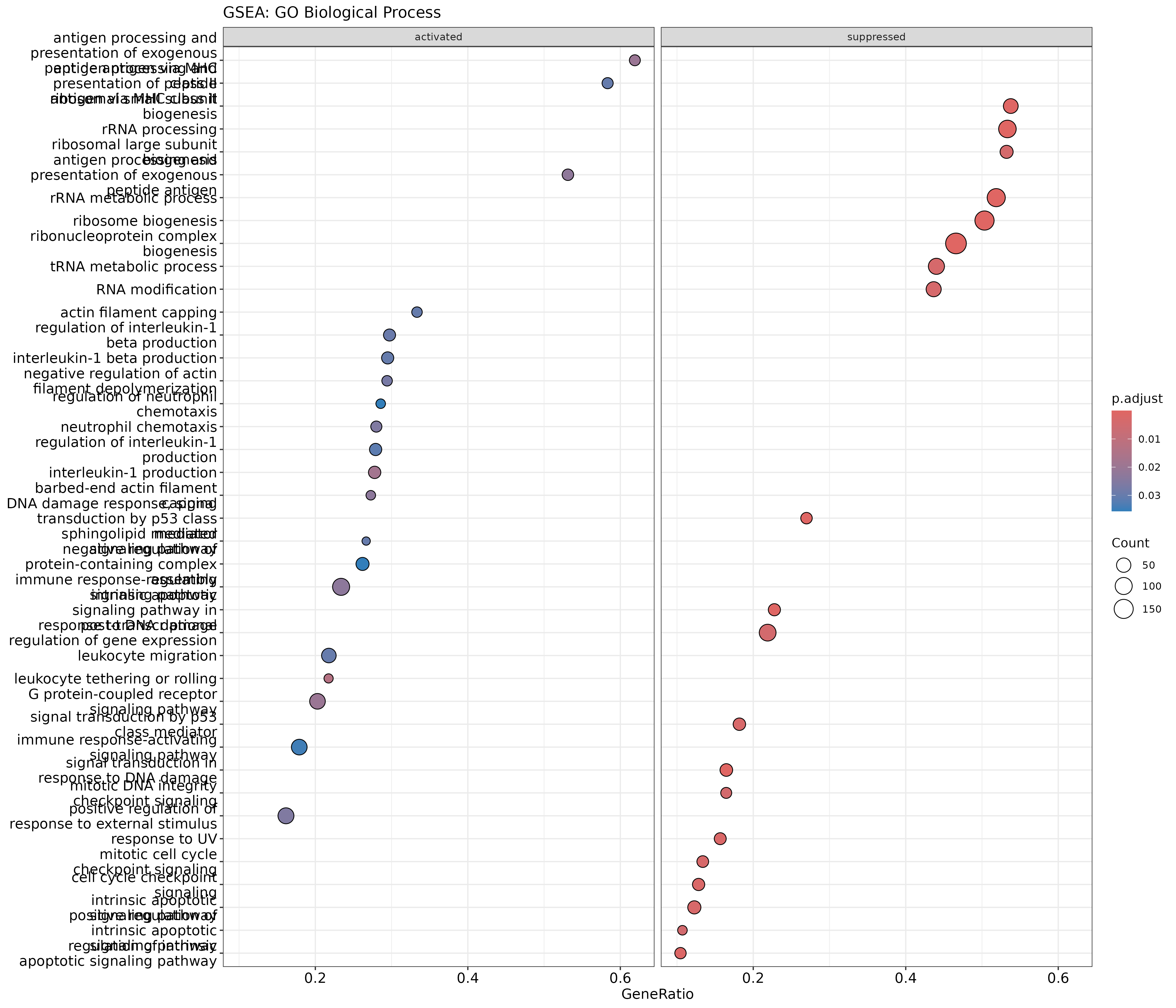
The .sign column indicates whether the gene set is
enriched in up-regulated (activated) or down-regulated
(suppressed) genes.
GSEA enrichment plot for a specific term
R
# Enrichment plot for top gene set
gseaplot2(gsea_go, geneSetID = 1, title = gsea_go$Description[1])
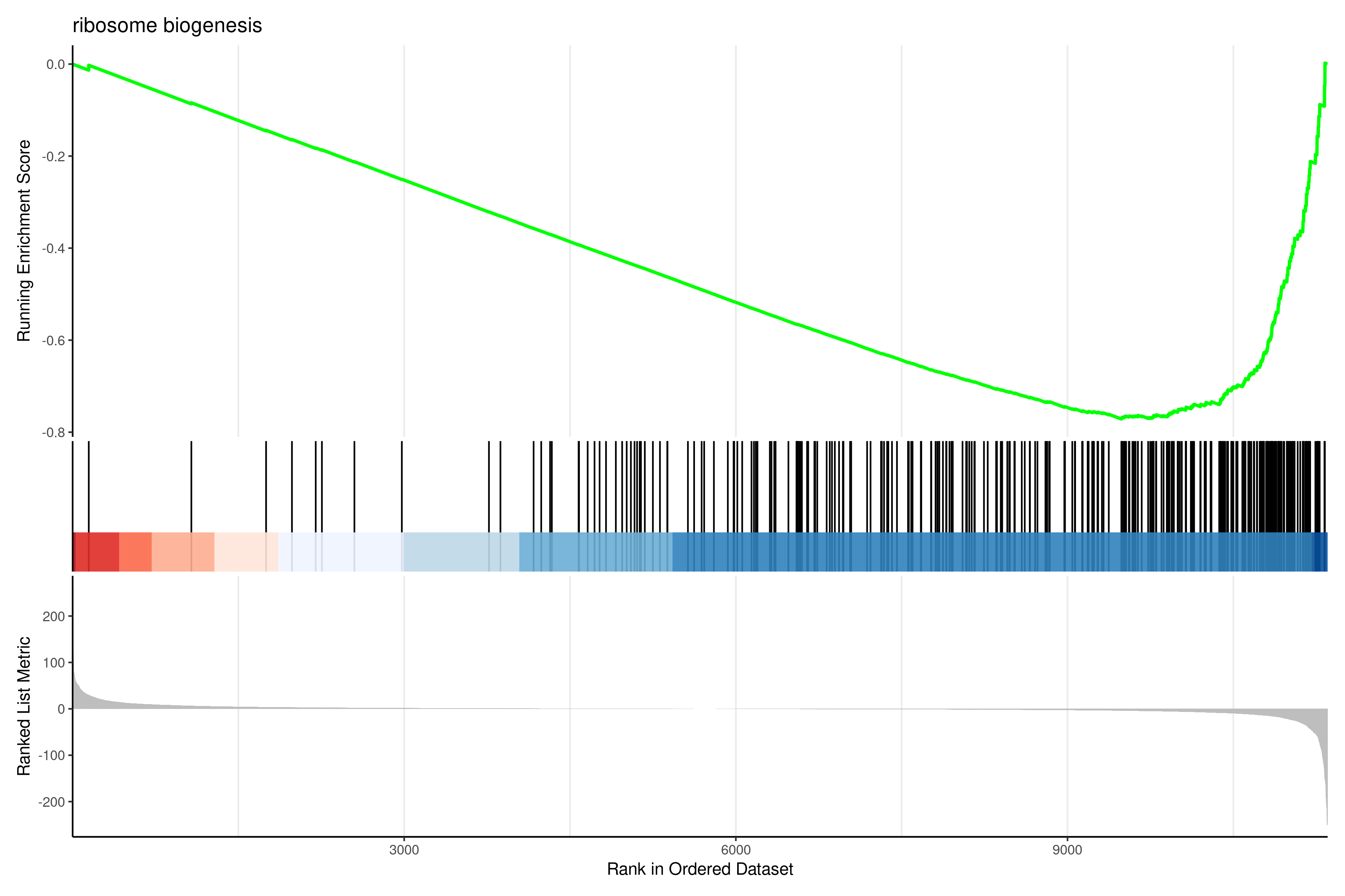
Interpreting GSEA results
Key metrics:
- NES (Normalized Enrichment Score): Direction and strength of enrichment. Positive = enriched in up-regulated genes; Negative = enriched in down-regulated genes.
- pvalue/p.adjust: Statistical significance.
- core_enrichment: Genes contributing most to the enrichment signal (“leading edge”).
GSEA is particularly valuable when:
- Changes are subtle but coordinated across many genes.
- You want to avoid arbitrary significance cutoffs.
- You’re comparing with published gene signatures.
Exercise: Compare ORA and GSEA results
- Do the same pathways appear in both ORA and GSEA results?
- Does GSEA identify any pathways that ORA missed?
- For pathways appearing in both, is the direction (NES sign) consistent with the ORA direction analysis?
Expected observations:
- Many top pathways should overlap between ORA and GSEA.
- GSEA may identify additional pathways where changes are subtle but coordinated.
- The NES sign (positive/negative) should match whether the pathway was enriched in up- or down-regulated genes in ORA.
- Discrepancies may indicate pathways where the signal comes from many small changes rather than a few large ones.
Step 6: Save results
Save all enrichment results:
R
# Create output directory
dir.create("results/enrichment", showWarnings = FALSE)

# GO results
write_csv(as.data.frame(ego_bp), "results/enrichment/GO_BP_enrichment.csv")
write_csv(as.data.frame(ego_bp_simple), "results/enrichment/GO_BP_simplified.csv")

# KEGG results
write_csv(as.data.frame(ekegg), "results/enrichment/KEGG_enrichment.csv")

# Hallmark results
write_csv(as.data.frame(ehall), "results/enrichment/Hallmark_enrichment.csv")

# Direction-aware results
write_csv(as.data.frame(ego_up), "results/enrichment/GO_BP_up_regulated.csv")
write_csv(as.data.frame(ego_down), "results/enrichment/GO_BP_down_regulated.csv")

# GSEA results
write_csv(as.data.frame(gsea_go), "results/enrichment/GSEA_GO_BP.csv")
Save plots:
R
# GO dotplot
pdf("results/enrichment/GO_BP_dotplot.pdf", width = 10, height = 8)
dotplot(ego_bp_simple, showCategory = 20) +
    ggtitle("GO Biological Process enrichment")
dev.off()

# KEGG barplot
pdf("results/enrichment/KEGG_barplot.pdf", width = 10, height = 6)
barplot(ekegg, showCategory = 15) +
    ggtitle("KEGG pathway enrichment")
dev.off()

# Hallmark dotplot
pdf("results/enrichment/Hallmark_dotplot.pdf", width = 10, height = 8)
dotplot(ehall, showCategory = 20) +
    ggtitle("MSigDB Hallmark enrichment")
dev.off()
Interpretation guidelines
Signs of meaningful enrichment
Enrichment results are more reliable when:
- Multiple related terms appear (not just one isolated hit).
- Consistent themes emerge across databases.
- Biological plausibility: Results align with known biology of your system.
- Reasonable gene counts: Terms with many genes (>5-10) are more robust.
- Moderate p-values: Extremely low p-values (e.g., 10^-50) may indicate annotation bias.
Common pitfalls
- Over-interpretation: A significant p-value doesn’t prove causation.
- Ignoring effect size: A term with 3/1000 genes is less meaningful than 30/100.
- Cherry-picking: Report all significant results, not just expected ones.
- Universe mismatch: Using wrong background inflates or deflates significance.
- Outdated annotations: Gene function annotations improve over time.
Summary
- ORA tests if gene sets contain more DE genes than expected by chance using the hypergeometric test.
- The background universe must include all genes that could have been detected as DE.
- Multiple testing correction (FDR) is essential when testing thousands of gene sets.
- GO provides comprehensive but redundant functional annotation; use
simplify()to reduce redundancy. - KEGG provides curated pathway maps but has limited gene coverage and requires Entrez IDs.
- MSigDB Hallmark sets offer 50 high-quality, non-redundant biological signatures.
- Direction-aware analysis (up vs. down separately) often reveals clearer biological signals.
- GSEA avoids arbitrary cutoffs by using the full ranked gene list; it detects subtle but coordinated changes.
- Convergent findings across multiple databases and methods strengthen biological interpretation.
- Always report methods, thresholds, and full results for reproducibility.